Lab 1 - EE 420L: Engineering Electronics II
For this first lab simulate, and verify the simulation
results with experimental measurements, the circuits seen in Figs. 1.21, 1.22,
and 1.24 (use a 1 uF cap in place of the 1 pF cap) of the book. Your results
should be similar to, but more complete than, the simulation results seen on
pages 17 - 23. In your report, and for each circuit, show the
·
Circuit schematic showing values and simulation
parameters (snip the image from LTspice).
·
Hand calculations to detail the circuit's
operation.
·
Simulation results
using LTspice verifying hand calculations.
·
Scope waverforms verifying simulation
results and hand calculations.
·
Comments on any differences or further potential
testing that may be useful (don't just give the results, discuss them).
Experiment 1: Circuit Fig 1.21
The circuit in Figure 1 below is an RC circuit with a 1V
input at 200Hz connected to a 1kΩ resistor in series with a 1µF
capacitor. This circuit and the two circuits following this experiment were all
simulated in LT Spice to obtain simulated values to be compared to hand
calculated theoretical values and experimental values obtained in the
laboratory.

Figure 1
The theoretical values hand calcluated will be below in
figure 2.

Figure 2
The simulation results from spice will be below in figure
3. As can be seen the magnitude of Vout
is .622 volts the phase is -51.48 degrees and the time delay is .909us.

Figure 3
Below in figure 4 is the experimental resluts of the circuit
in figure 1.21 from the book. From figure
4 the result of the time delay is displayed at -47.11 degress and estimating
the time delay using 20us/division the resulting time delay is roughly 600us.
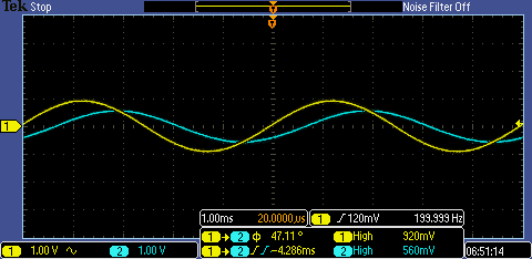
Figure 4
Below in table 1 is the consolidation all of the pertinant
information aquired from each result above.
|
Fig 1 |
Magnitude (V) |
Phase Shift
(Degrees) |
Time Delay (uS) |
|
Simulation |
.622 |
-51.49 |
909 |
|
Theoretical |
.622 |
-51.48 |
715 |
|
Experimental |
.560 |
-47.11 |
600 |
Table 1
Experiment 2: Circuit Fig 1.22
The circuit in figure 5 is similar to the RC circuit in Fig.
1 with the addition of a 2µF capacitor in parallel with the 1kΩ resistor.
Theoretically, the capacitor in parallel with the resistor should reduce the
amount of loss in the strength of the signal when compared to the circuit in
experiment one. The same process will be used as in experiment one to compare
values and analyze results. The comparison of values will be
included in a table following the images containing the relevant quantities
measured during each different type of analysis.
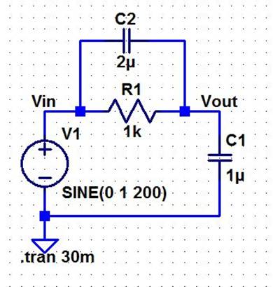
Figure 5
The theoretical hand calculations for the schematic in figure
5 above will be below in figure 6.
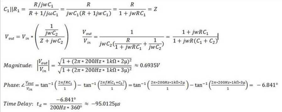
Figure 6
The spice simulation results for circuit seen in figure 5
will be below in figure 7. As can be
seen the Magnitude of Vout is .693 Volts the phase is -6.84 degrees and the
time delay is 72us and the 3db frequency is 158.7Hz.

Figure 7
Below in figure 8 is the experimental resluts of the circuit
from figure 5 implemented on a breadboard.
As can be seen the phase is -4.478 degrees the magnitude of Vout is
640mV and the time delay is 103.2us.
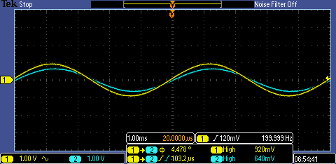
Figure 8
Below in table 2 will be the consolidated pertinant
information gathered from the results of experiment from figure 5.
|
Fig 2 |
Magnitude (V) |
Phase (degrees) |
Time Delay (uS) |
|
Theoretical |
0.6935 |
-6.841 |
-95 |
|
Simulation |
0.6935 |
-6.841 |
-72 |
|
Experimental |
0.640 |
-4.478 |
-103.2 |
Table 2
Experiment 3: Circuit Fig 1.24
The circuit in figure 9 is the same
as the circuit in experiment one, but for experiment three the input has been changed
to a pulse. Using the pulse will allow calculation of the delay time and the
rise time of the signal. The results of the analysis are displayed in the
images below. The measured values will be displayed in a table below.
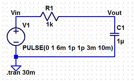
Figure 9
The theoretical hand calculations for the schematic in figure
9 above will be below in figure 10.
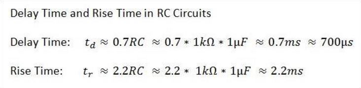
Figure 10
The spice simulation results for circuit seen in figure 9
will be below in figure 11. As can be
seen the time delay is 695.99uS and the rise time is 2.155mS.

Figure 11
Below in figure 12 is the experimental resluts of the circuit from figure
9 implemented on a breadboard. As can be
seen the measurment tool displays a time delay of 800us. and a rise time of
roughly 2ms. The error is due to human
error using the O-Scope.
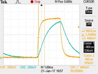
Figure 12
Below in Table 3 will be a consolidated table of pertinant date retrieved in
the experiment above. As can be seen the
results are fairly close excluding the time delay of the experimental value
which was due to human error using the O-Scope.
|
Figure 9 |
Delay Time (uS) |
Rise Time (mS) |
|
Theoretical |
700 |
2.2 |
|
Simulation |
695.99 |
2.155 |
|
Experimental |
800 |
2 |
Table 3
For the AC response seen in Fig. 1.23 of the book generate a table showing
some representative measurement results (frequency, magnitude, and phase). Below in figure 13 is the results of several
measurments taken.

Figure 13
Below in table 4 is the consolidated information collected above from the
simulation results. The following
information in the table is known as the frequency response of the system
obtained from the boding plots above in figure 13.
|
Frequency (Hz) |
Magnitude (db) |
Phase (degrees) |
|
159 |
-3 |
-45 |
|
200 |
-4 |
-51 |
|
278 |
-6 |
-60 |
|
620 |
-12 |
-75 |
|
10K |
-36 |
-90 |
Table 4
Conclusion:
The experiments performed in Laboratory One offered the opportunity to
review basic RC circuits, to practice LT Spice simulations and to compare the
values obtained via different methods of analysis, specifically
experimentation, hand calculation and simulation. The laboratory results also
demonstrated the variances that may occur within the different methods of
analysis due to different means of measuring inherent in each technique.
Return to Dr.
Baker’s Course Listings