Lab

Lab 1 - EE 420L

Authored by Sharyn Miyaji,

Wednesday, January 25, 2017

Pre-Lab Work

Learn how to edit webpages
Review Lab 1 prior to lab

Lab Work

Figure 1.21

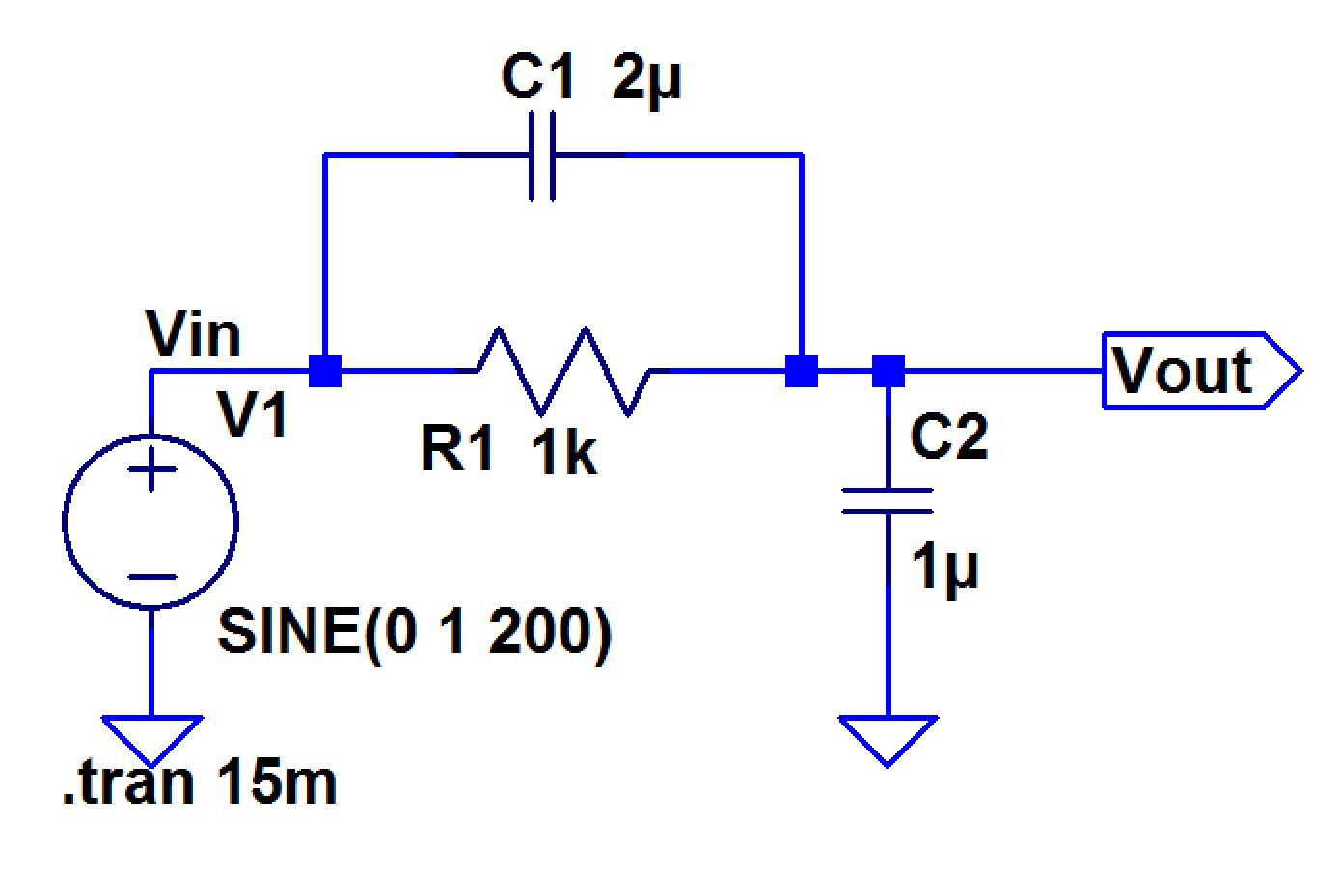
Schematic

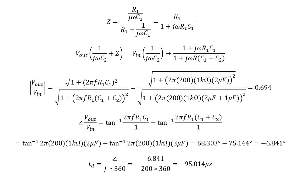
Hand-Calculation

Note: Time delay is negative since the output is lagging from the input.

LTspice Simulation

Scope Measurements

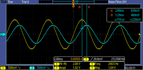
To measure the time delay between the voltage input and output for the simulation, the peak of both the input and output voltage must be found. Once that is found, the time difference between those two points is the time delay. In this case, the peak voltage of the input is 1 volts and the calculated peak voltage of the output is about 0.623 volts. When the time is measured at both of those points in the LTspice simulation and scope measurements , the difference is taken which is measured about 720 us and closely matches the hand calculations.

Figure 1.22

Schematic

Hand-Calculation

Note: Again, the time delay is negative because the output is lagging the input.

LTspice Simulation

Scope Measurements

http://cmosedu.com/jbaker/courses/ee420L/s17/students/miyajis/lab1/Fig1.22_Results.JPG

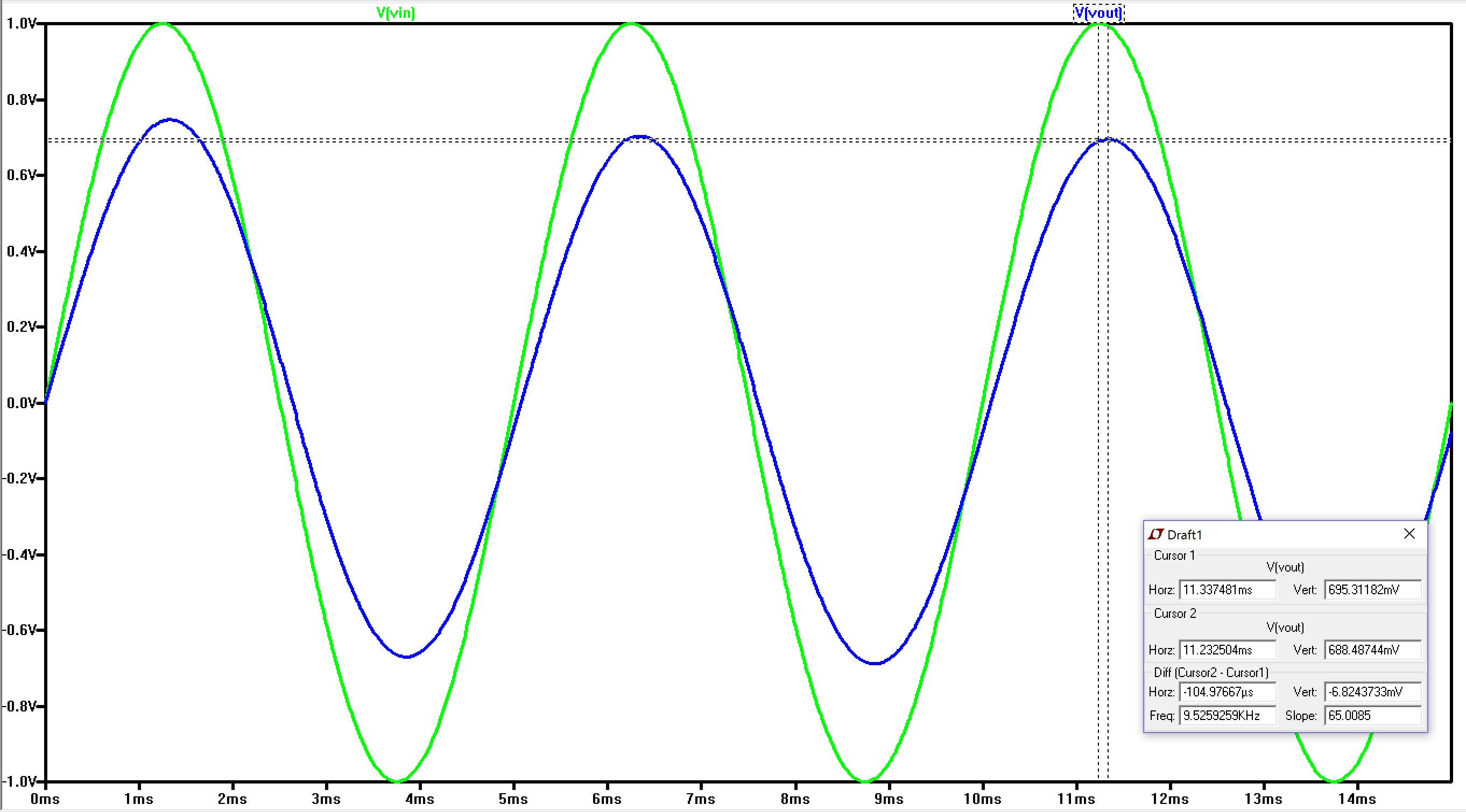
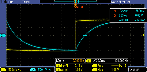
Same as Figure 1.21, the time delay is measured based on the peak voltage of the input and the peak voltage of the output. Based on the hand calculation, the time delay is about 95 us, which is close to the measured values in both simulations.

Figure 1.24

For this figure, the capacitor has changed from 1pF to 1uF.

Schematic

http://cmosedu.com/jbaker/courses/ee420L/s17/students/miyajis/lab1/Fig1.24_schematic.JPGhttp://cmosedu.com/jbaker/courses/ee420L/s17/students/miyajis/lab1/Fig1.24_schematic.JPG

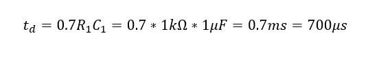
Hand-Calculation

LTspice Simulation

Scope Measurements

http://cmosedu.com/jbaker/courses/ee420L/s17/students/miyajis/lab1/Fig1.24_Results.JPG

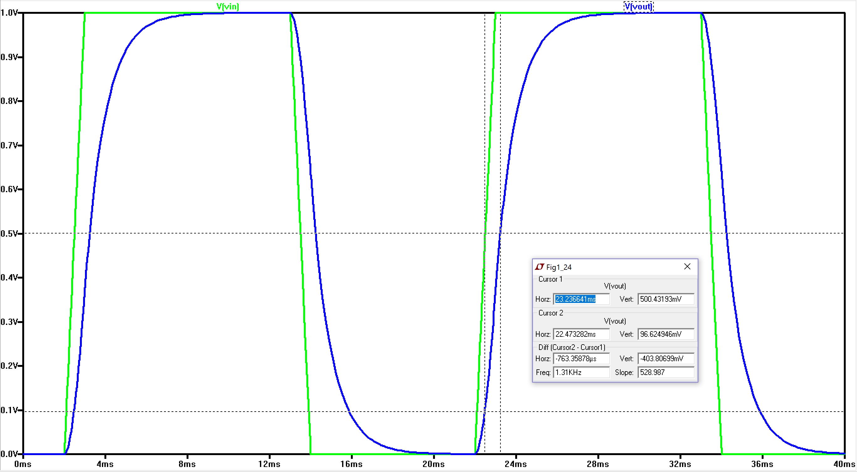
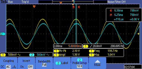
For this circuit, time delay is being calculated and measured, which is found at the halfway point of the input voltage. Since the value of the capacitor was increased, the pulse setting of the circuit is increased as well. To get as accurate of a result, the pulse width must be long enough for the capacitor to charge and discharge fully. Based on the hand calculation, the time delay should be about 700 us. The LTspice simulation is off by about 60 us, which is not a lot, and the oscilliscope measurement is very close to the hand calculation.

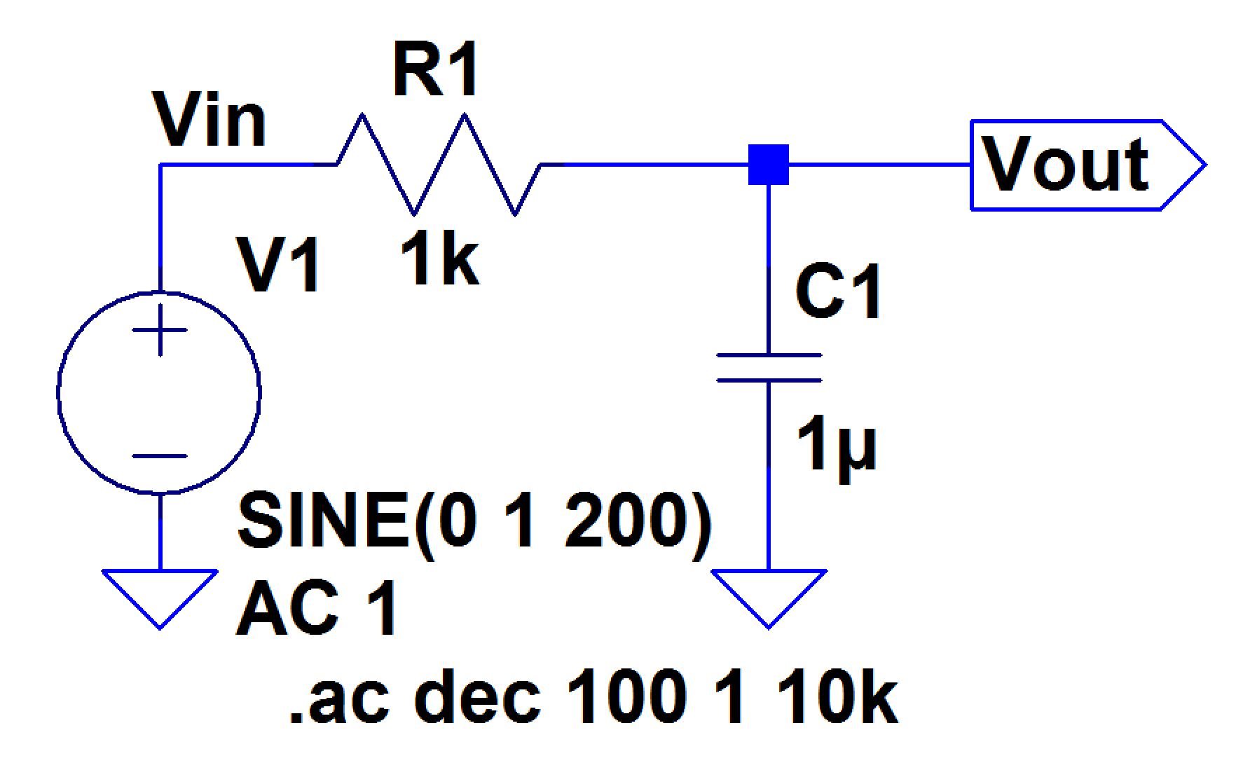
Figure 1.23

Schematic

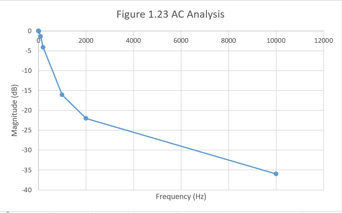
AC Analysis Sketch

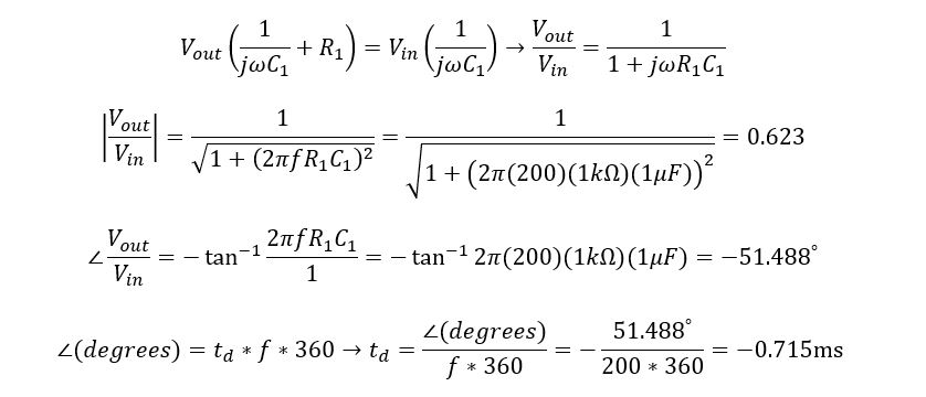
http://cmosedu.com/jbaker/courses/ee420L/s17/students/miyajis/lab1/Fig1.23_Sketch.JPG

Using the equations from Figure 1.21, the following magnitude and phase angle in degrees have been calculated based on the varing frequencies. Since the magnitude is in decibels, the voltage magnitude must be converted using the following equation, V(dB) = 20*log(|Vout/Vin|)

Hand Calculations

Frequency (Hz)	Magnitude (dB)	Phase Angle (degrees)
1	-171u	-359m
2	-686u	-720m
10	-17.1m	-3.595
20	-68.0m	-7.162
100	-1.445	-32.142
200	-4.110	-51.488
1k	-16.072	-80.957
2k	-22.012	-85.450
10k	-35.965	-89.088

After the calculations have been made, the magnitudes and phase angles are estimated in the plot for comparison to the hand calculations by probing the LTspice simulation with respect to the frequencies.

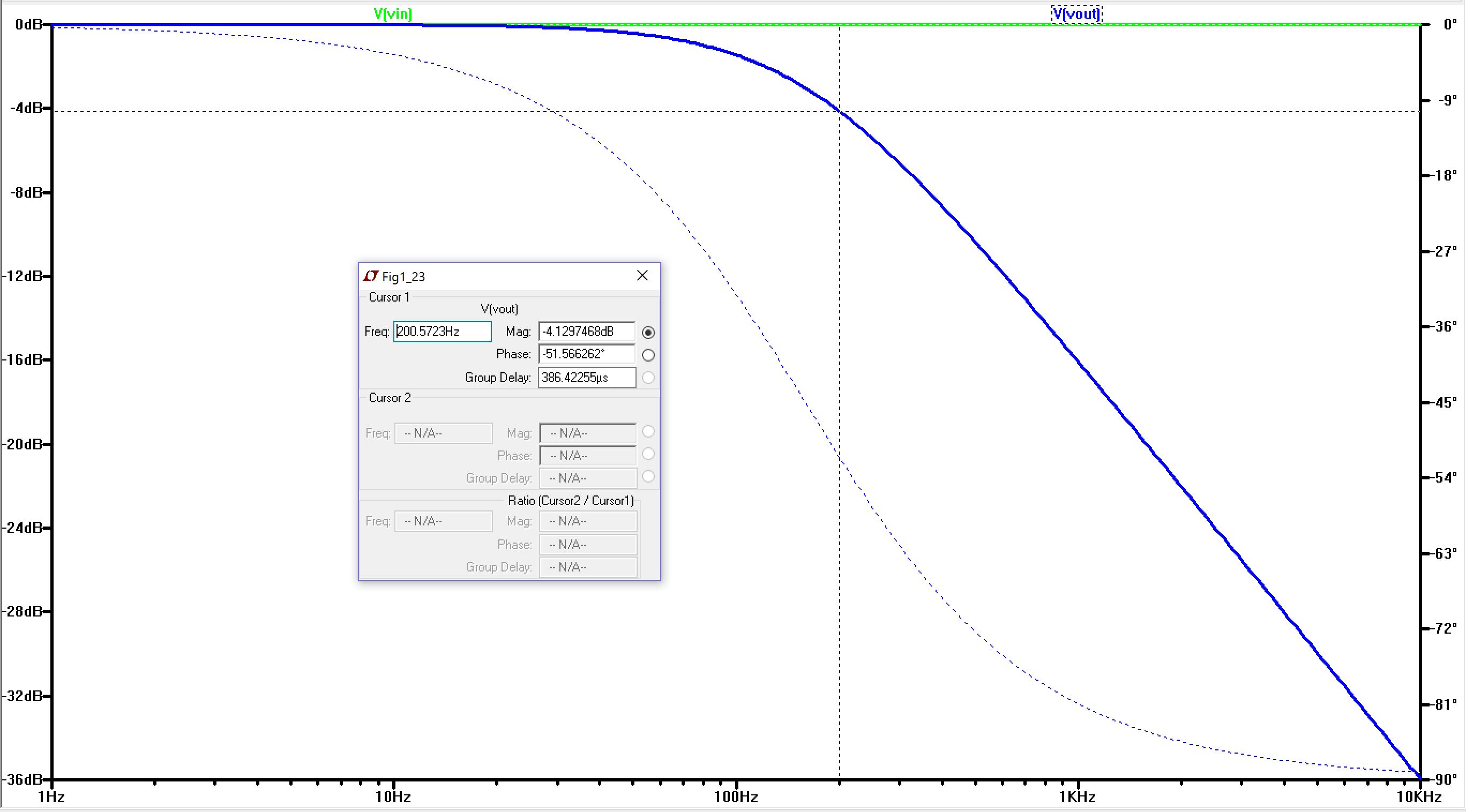
LTspice Simulation

LTspice Results

Frequency (Hz)	Magnitude (dB)	Phase Angle (degrees)
1	-171u	-360m
2	-686u	-720m
10	-16.98m	-3.580
20	-68.341m	-7.1778
100	-1.465	-32.347
200	-4.130	-51.566
1k	-16.105	-80.992
2k	-22.060	-85.475
10k	-35.965	-89.088

Between the theoretical and actual of the calculations and plots, the values and graphs are very similar to each other, even though the Excel plot is not scaled like the LTspice plot.

Back-Ups

I will be backing up my files on my Google Drive and my UNLV student drive.

Return to Sharyn's EE420L Labs

Return to EE 420L Labs