Lab

ECE 421L - Lab 1

John Huang

Huangj19@unlv.nevada.edu

Spring 2015

Lab description:

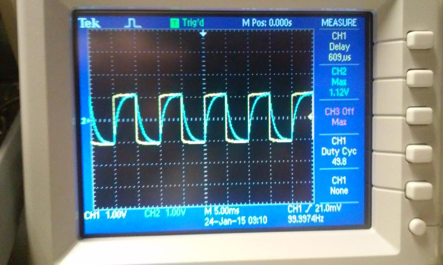
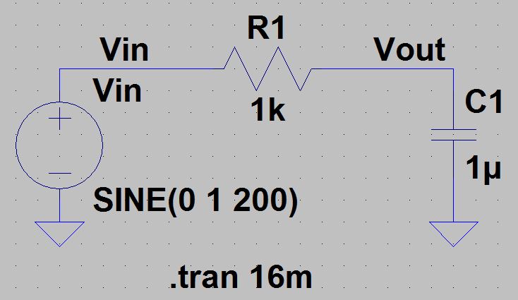
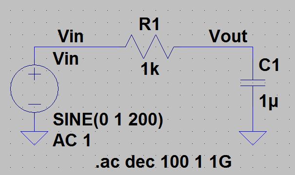
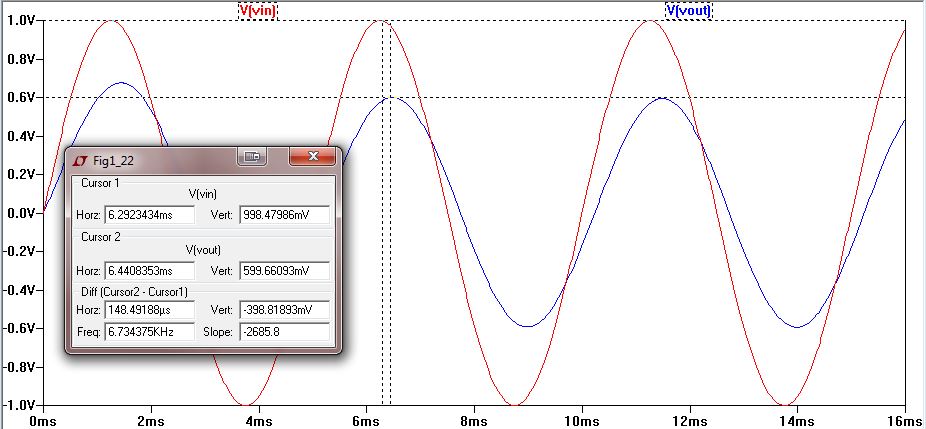
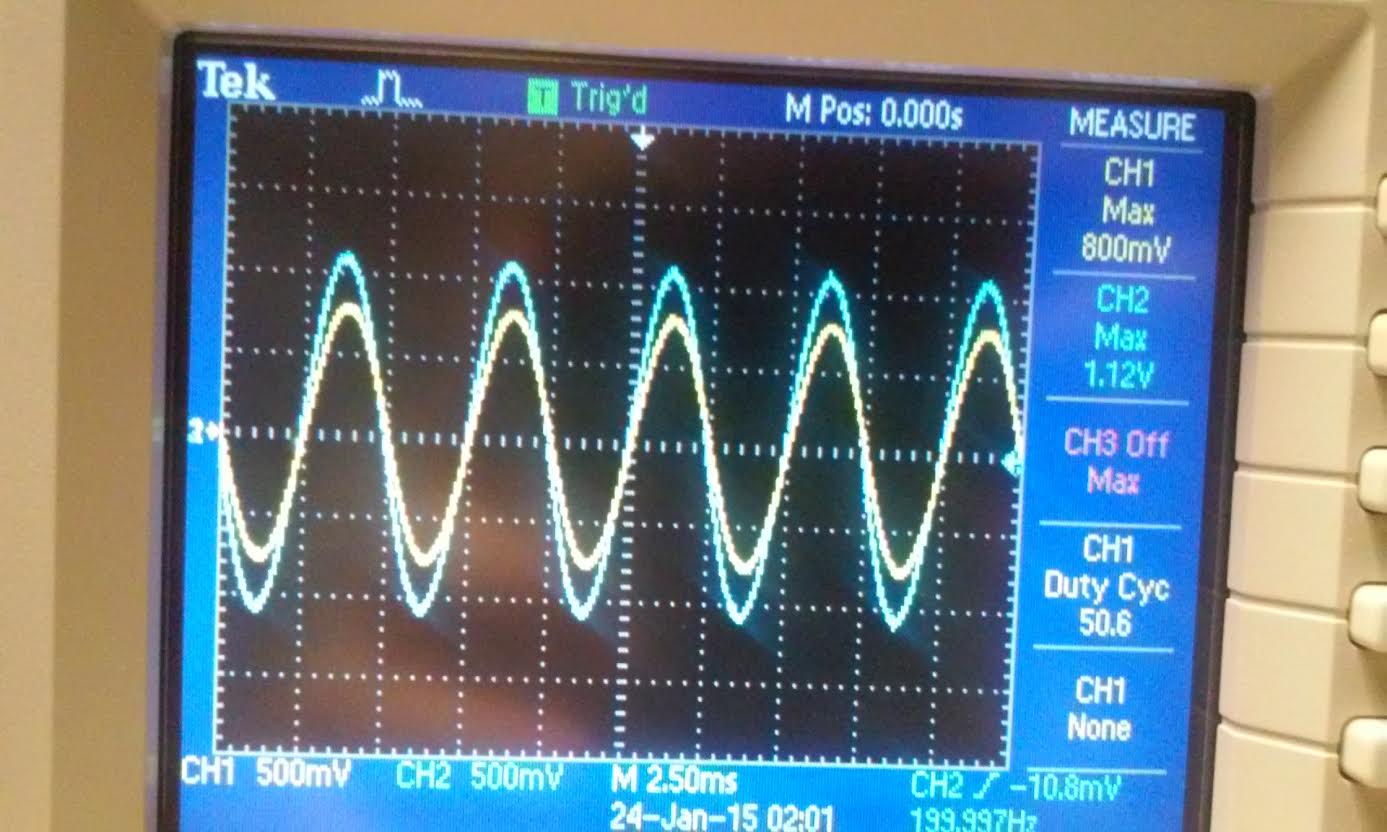
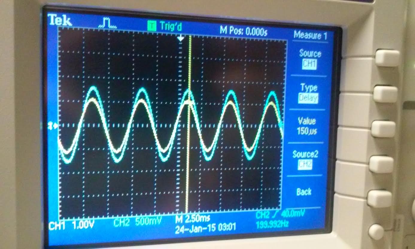
Lab 1 is used to verify the simulation results with experimental measures from the textbook.
Figures 1.21, 1.22, and 1.24 are used, we replace the 1pF capacitor with a 1uF capacitor.

Fig 1.21:
Schematic:

transient	ac sweep

Hand calculations:
magnitude:
|Vout/Vin| = 1/sqrt((1+2*pi*f*R*C)^2)) = 0.623 V

phase:
theta = -arctan((2*pi*f*R*C)/1) = 51.5 degrees

delay:
td = theta/(f*360) = 715 us

Simulations:
The simulation provides us both the input voltage and the output voltage. We are able to compare both the magnitude difference and delay of the output voltage.
We can see that the transient response simulation gives us a fairly accurate time delay (705us) and magnitude(0.623V) for the output voltage.

transient	ac sweep

The ac sweep provides us the frequency response of the circuit.
We can see that at 200 Hz, we get the calculated magnitude and phase for the RC circuit above.

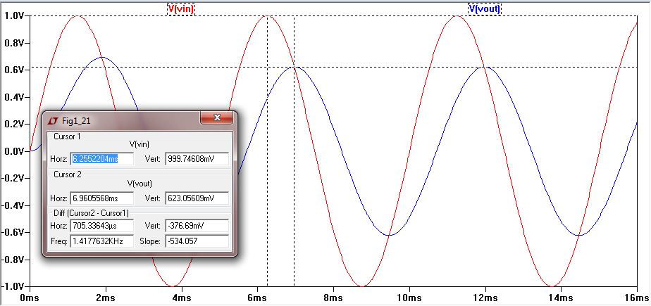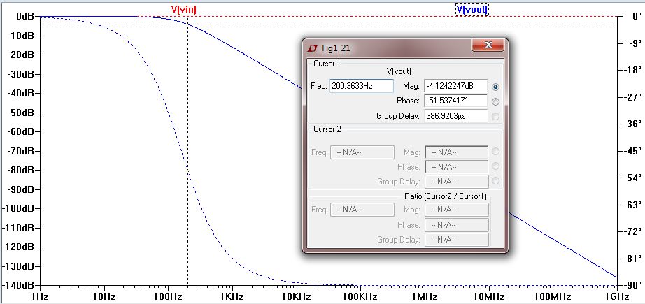Frequency (Hz)	Magnitude (dB)	Phase (degree)
1	0	0
10	0	-3.7
100	-1.55	-33.2
200	-4.1	-51.53
1k	-16.3	-81.2
10k	-36.5	-89.1
100k	-55.9	-89.9
1M	-76	-90

Scope waveforms:
Here are the waveforms from the oscilloscope that shows the magnitude at 700mV which is close to the theoretical magnitude of 623mV.
While the delay is not as close being only 620us compared to the theoretical 715us.

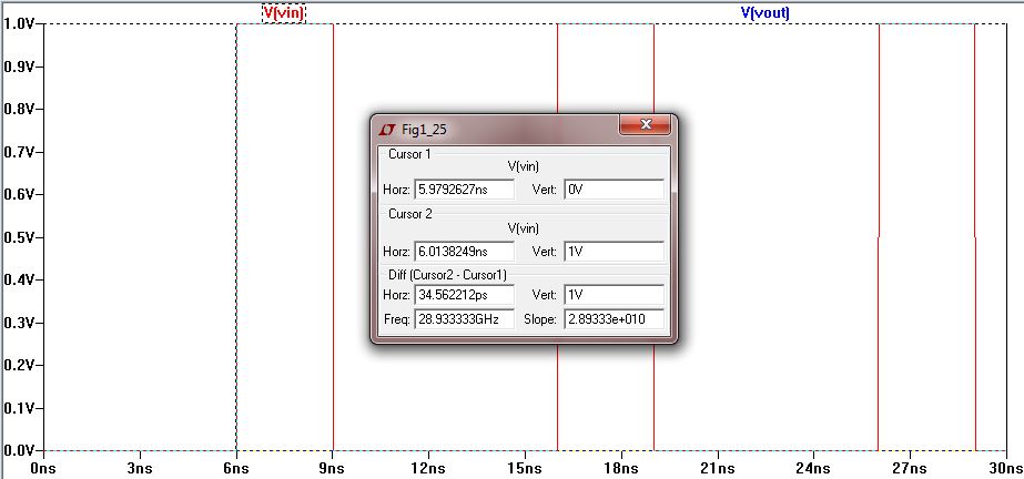
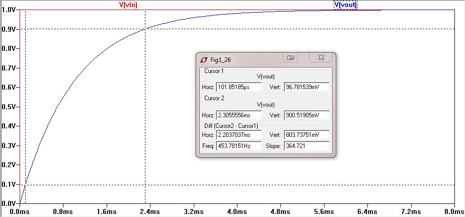
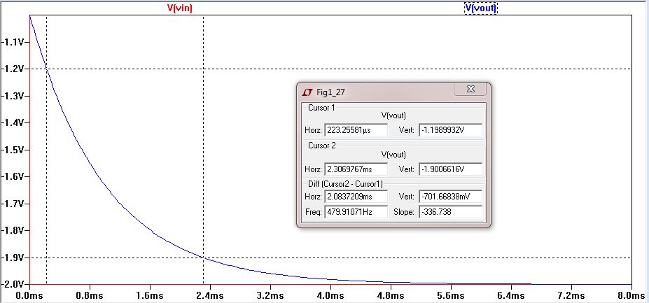
magnitude	time delay

These waveform results could be improved if we picked resistor and capacitor values extremely close to the values in the schematic. This issue is very common because of the variance of each component from the manufacture.

Fig 1.22:
Schematic:

http://cmosedu.com/jbaker/courses/ee420L/s15/students/huangj19/lab1/5.JPG

Hand calculations:
magnitude:
|Vout/Vin| = sqrt(1+(2*pi*f*R*C1)^2)/sqrt(1+(2*pi*f*R*(C1+C2))^2) = 0.6 V

phase:
theta = arctan((2*pi*f*R*C1)/1) - arctan((2*pi*f*R*(C1+C2))/1) = -6.82 degrees

delay:
td = theta/(f*360) = -95 us = 95us (there is no such thing as negative time!)

Simulations:
Here we see that the delay seen in the simulation is a bit off from the calculated delay, approximately 50us longer delay, however the magnitude is pretty much on point.

http://cmosedu.com/jbaker/courses/ee420L/s15/students/huangj19/lab1/6.JPG

Scope waveforms:
For the magnitude, we see that the input voltage is at 1.12V while the output voltage is at 800mV. If you consider the difference of 120mV through the waveforms, we would get an output voltage of 680mV which is close to the theoretical 600mV.
The time delay is very off, almost 50% extra delay.

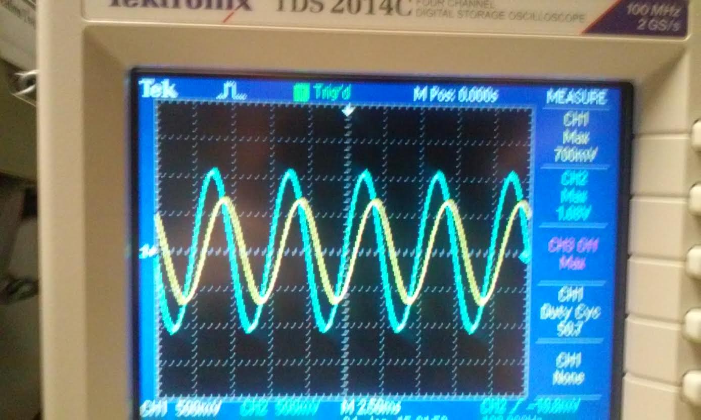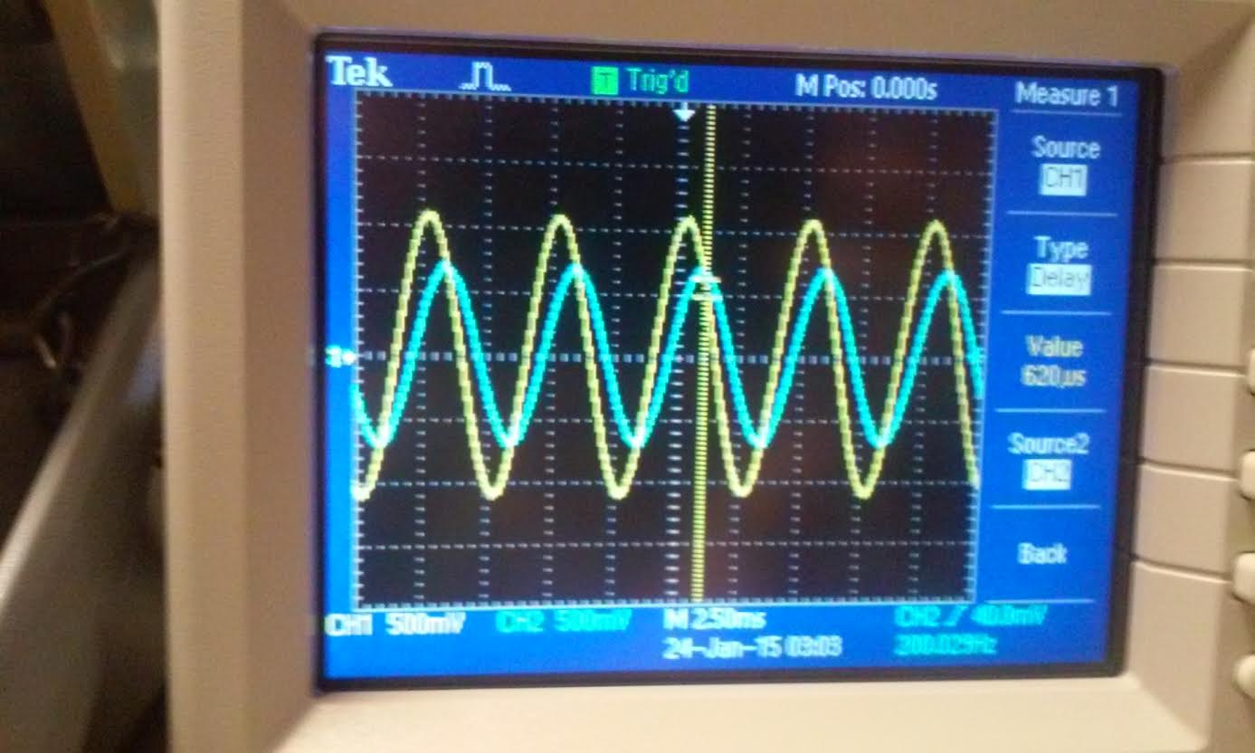magnitude	time delay

These issues might be adjusted by using better components as stated previously. Retesting these values to make sure that the magnitude of the input voltage is 1V would also be required.

Fig 1.24:
schematic:
Here we are trying to see the difference in changing the rise and fall time of the pulse source.

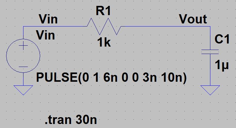
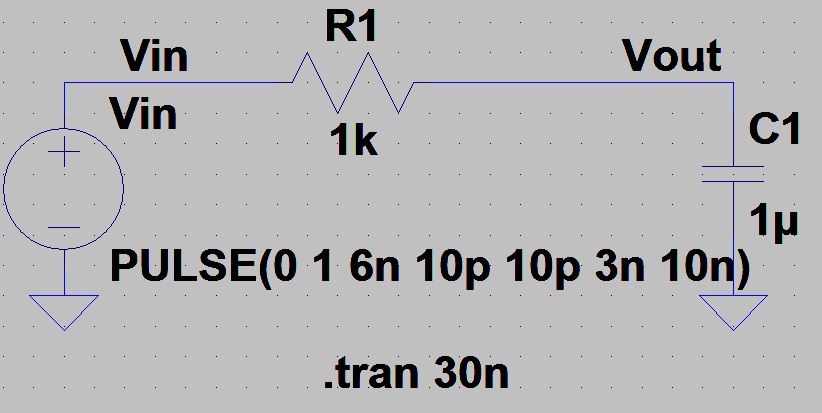
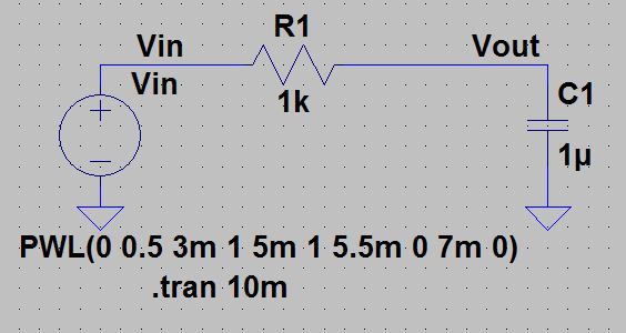
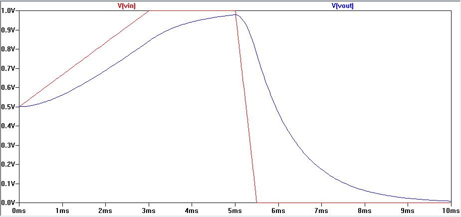
0s input pulse	10p input pulse

We use a pulse source to measure the delay and the rise time of an RC circuit, in order to get the fall time, we switch the polarity of the pulse wave.

time delay and rise time	fall time

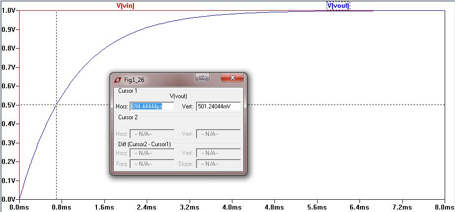
The piece-wise linear (PWL) source is useful if you want to specify arbitrary waveform shapes. You are able to set the voltage/current at specific points of time to change.
Here we have set the voltages of the PWL to the values of the table:

Time (ms)	Voltage (volts)
0	0.5
3	1
5	1
5.5	0
7	0

piece-wise linear (PWL) source

http://cmosedu.com/jbaker/courses/ee420L/s15/students/huangj19/lab1/18.JPG

Hand calculations:
td = 0.7*R*C = 700us
tr = tf = 2.2*R*C = 2.2ms

Simulations:
You can see that setting your own delay, rise and fall time can make a big difference in your simulations. Even though we set the rise and fall times to 0, it almost takes an order of magnitude for the simulation to rise and fall.
Once we set the rise and fall time to 10ps we can see how much faster it takes for the input voltage to change as we expect.

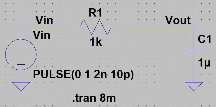
0s input pulse	10ps input pulse

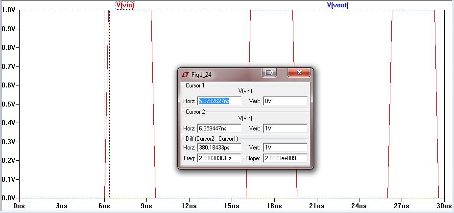The delay time and rise time are very accurate in both simulations, both being within the margin of error.
Note that we measure the delay time of the output voltage when it reaches 50% of the input voltage and we measure the rise time by the delta of the time it takes for the voltage to go from 10% to 90%.

delay time	rise time

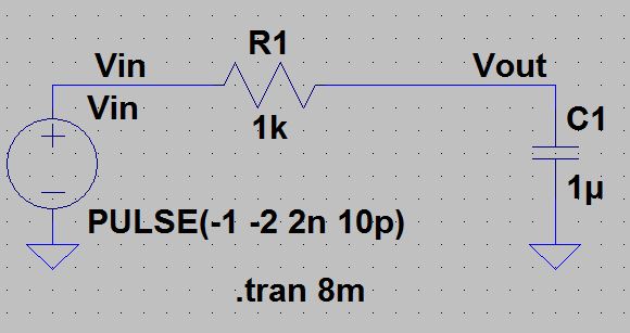
We measure the fall time in the exact opposite way as the rise time, going from 90% to 10% of the input voltage.
The piece-wise linear graph is an example of how you can input your own voltages at specific periods of time in order to obtain specific waveform shapes.

fall time	piece-wise linear source

Scope waveforms:
Here we have the waveform to measure the time delay of the circuit. The theoretical time delay was 700us, the waveform shows a delay time of 609us, about a 15% difference.

http://cmosedu.com/jbaker/courses/ee420L/s15/students/huangj19/lab1/1.24.jpg

Unforunately we were not able to measure the rise time and fall time of the RC circuit. That should be definitely done to further potential the testing of an actual circuit.

Conclusion:
From the lab we can tell the the hand caculations, ltspice simulations and the actual results are never exactly the same.
We can see that the simulations are always close to the theoretical hand calculations, however not the same can be said about the experimental results.
The most error comes from experimental results, which is caused by either human or component error. This is especially true when you are dealing with very small numbers and trying to get percise values.
Even in the ltspice simulations it is not easy to get the exact voltage to measure the time, etc...
Over all you can say that the hand calculations and the ltspice simulations give the best results, while the experimenal results have a varying amount of error.

Back up:
Make sure you back up your whole CMOSedu folder with all your labs by compressing the folder and sending it to yourself through email.

http://cmosedu.com/jbaker/courses/ee420L/s15/students/huangj19/lab1/20.JPG

Return to my lab reports

Return to student lab reports

Return to ee420L webpage