Lab 1 - EE 421L 

Authored by Isabella Paperno, paperi1@unlv.nevada.edu

Start date: 08/30/2023

Due date: 09/06/2023

Pre-lab work:

• Prior to the first day of the lab, but no earlier than one week before the lab starts, get a CMOSedu account, using your UNLV email address, from Dr. Baker, rjacobbaker@gmail.com
• Review the material seen here covering editing webpages (do this before the first lab)
  

Lab description:

We will familiarize ourselves with Cadence by following Tutorial 1 seen here up to the 25th image.

We will also use an Xterm (written and video) as discusssed in class and NOT a remote desktop as used in the tutorial.

Lab procedures:

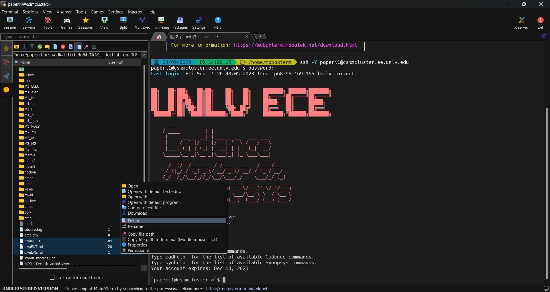
After setting Cadence up we need to go to the following directory: $HOME/ncsu-cdk-1.6.0.beta/lib/NCSU_TechLib_ami06

Then select and delete the divaDRC.rul, divaEXT.rul, and divaLVS.rul files.

Once those files are gone, extract files from diva_rul_files.zip and upload them into the $HOME/ncsu-cdk-1.6.0.beta/lib/NCSU_TechLib_ami06 directory.

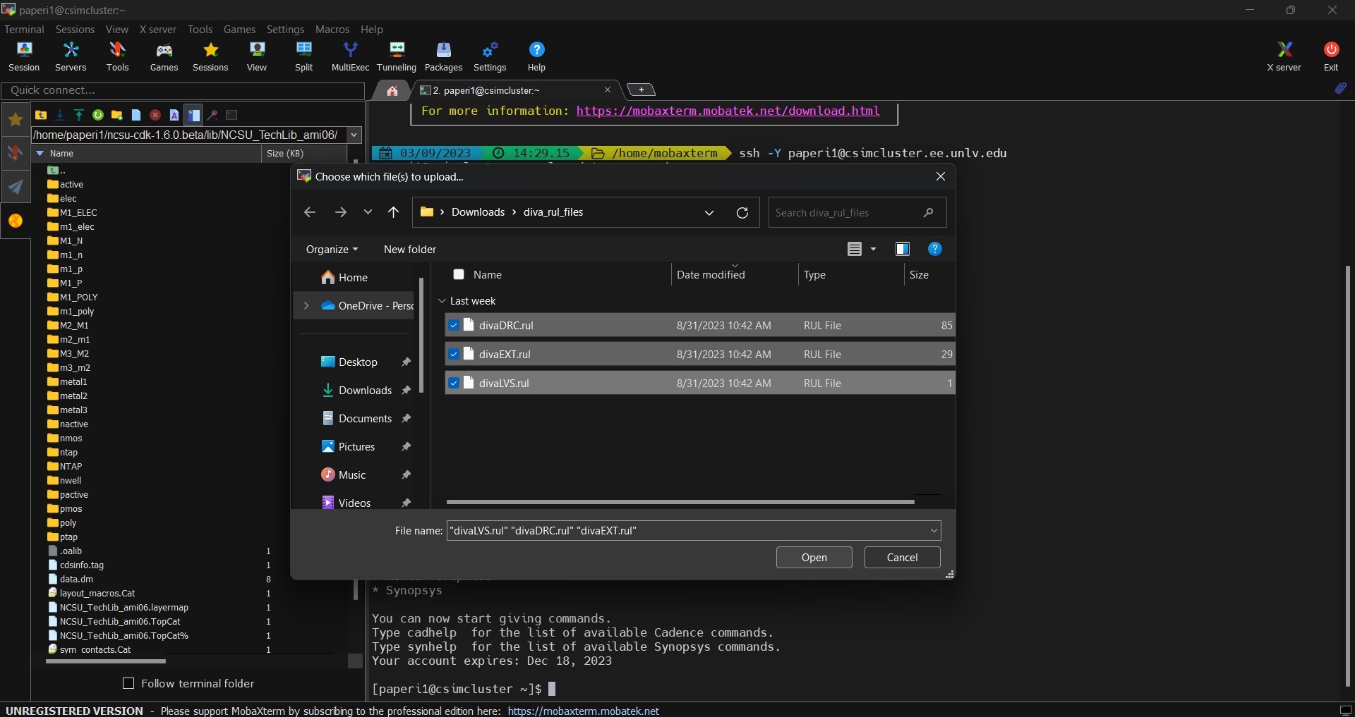
Upon completion of this we will be able to use DRC, Extract, and LVS on our layouts.

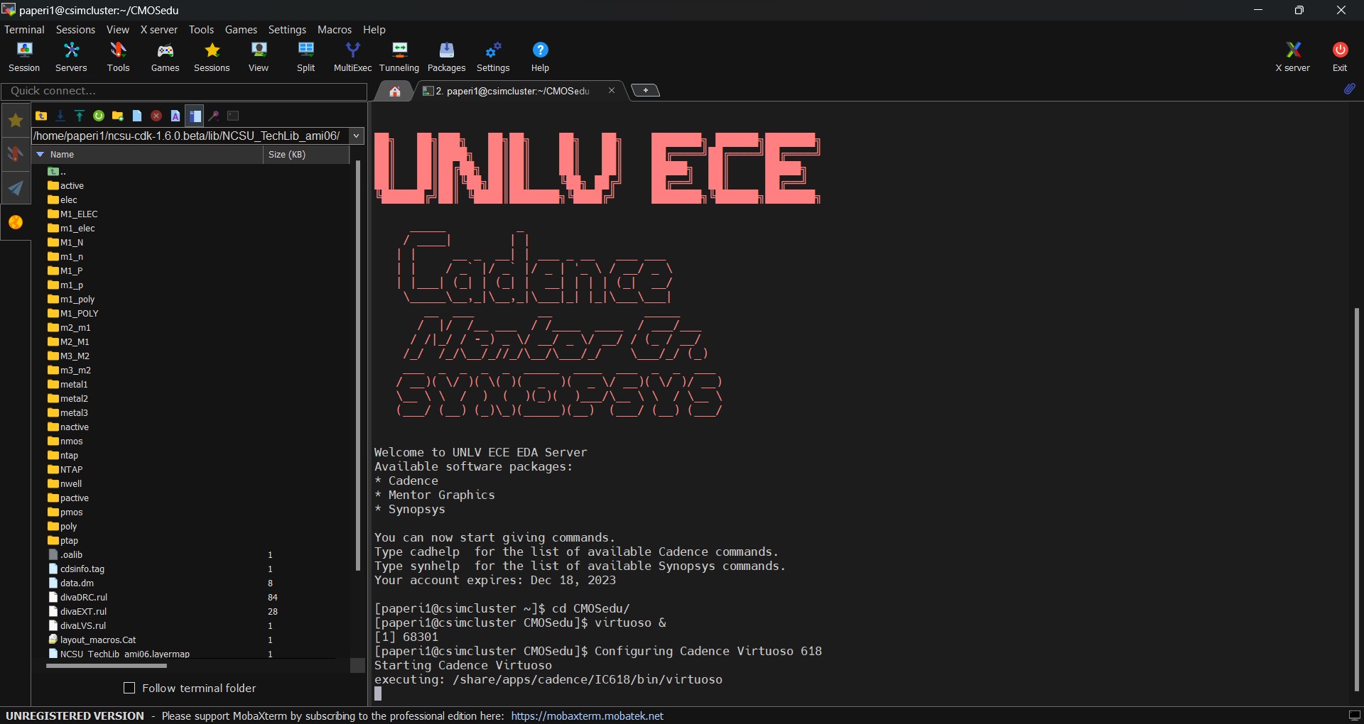
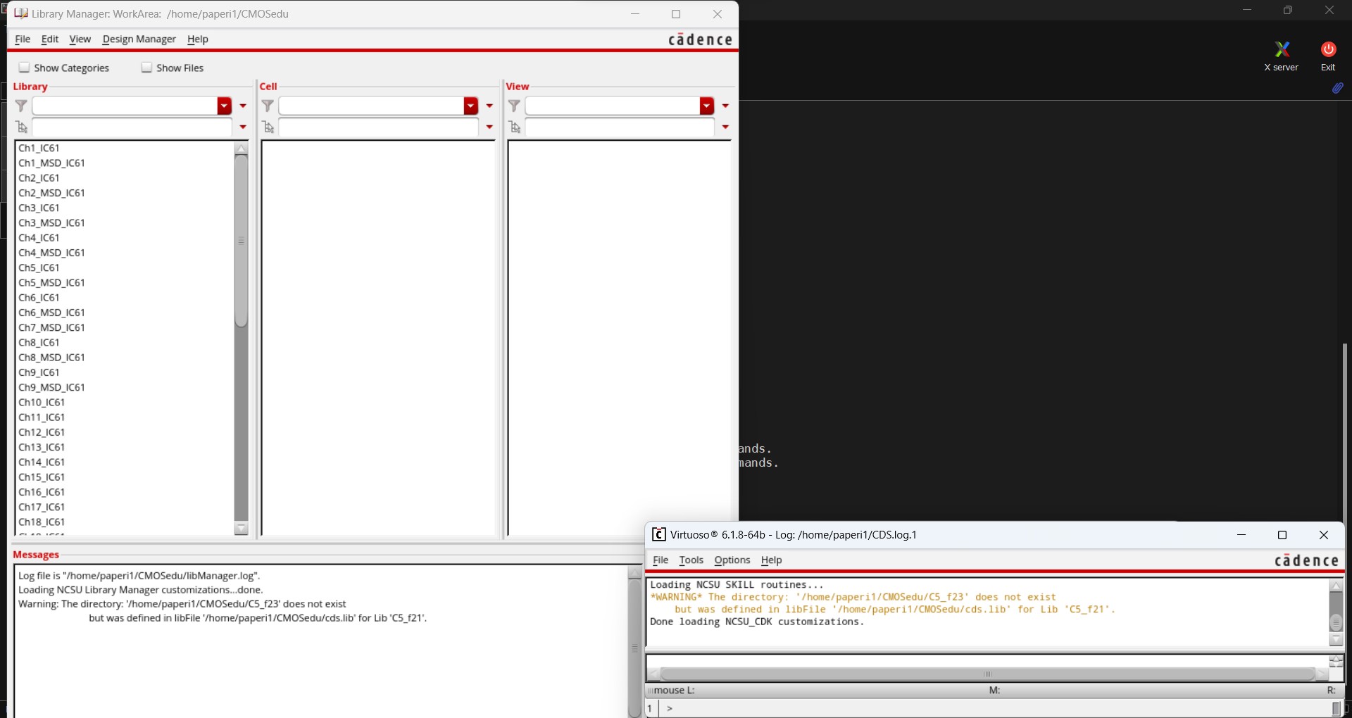
Doing so causes Virtuoso to open as the Command Interpreter Window (bottom right) then the Library Manager (left), all while keeping our terminal window open in the background.

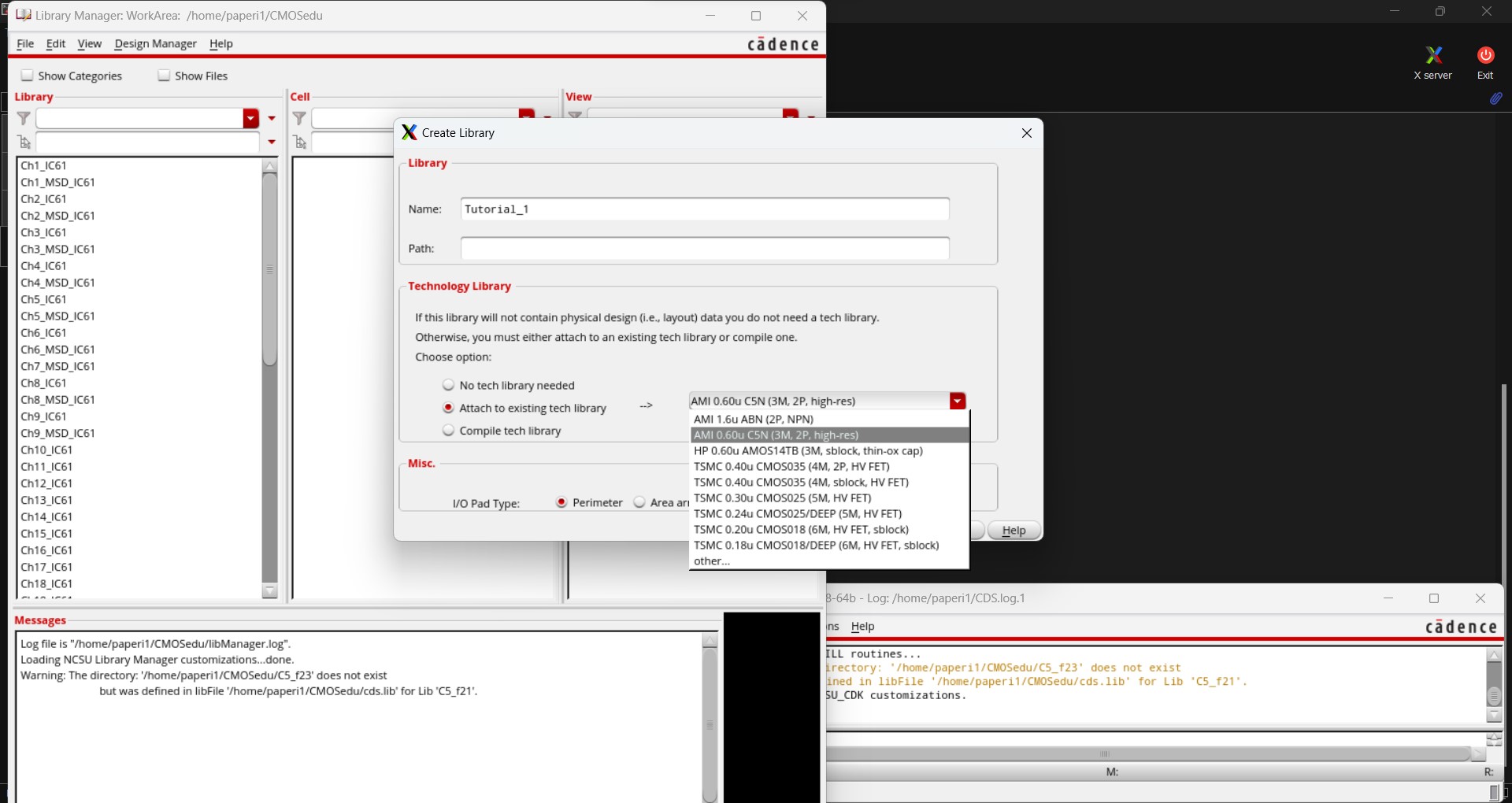
Now we can create a new library. To begin, go back to the Library Manager and select File -> New -> Library to have a window to create a new library pop up. We'll name the library Tutorial_1 then under the Technology Library select "Attach to exisiting tech library" and find the AMI 0.60u C5N (3M, 2P, high-res) selection. Once selected hit Apply then OK.

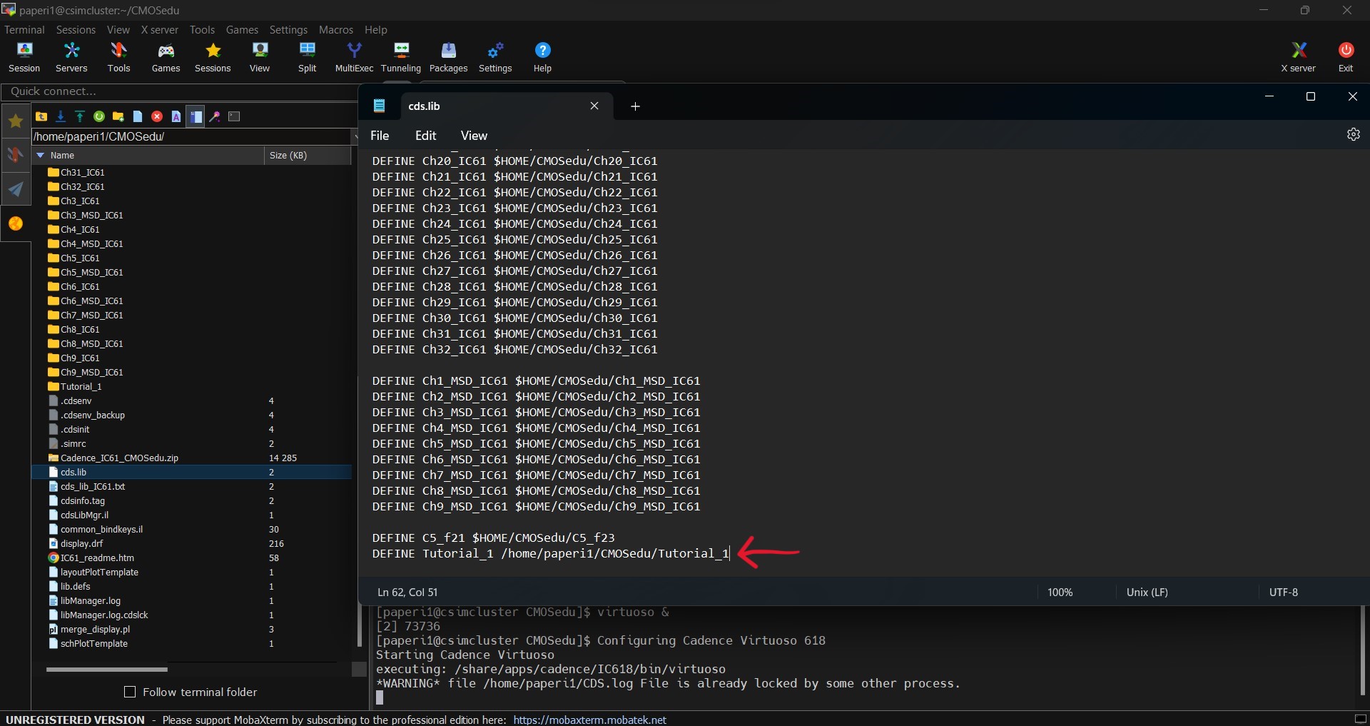
Any time a library is created, we need to define it in our cds.lib file. To do so, go back into the CMOSedu directory and open the cds.lib file. Scroll to the very bottom of the file and add DEFINE Tutorial_1 /home/paperi1/CMOSedu/Tutorial_1.

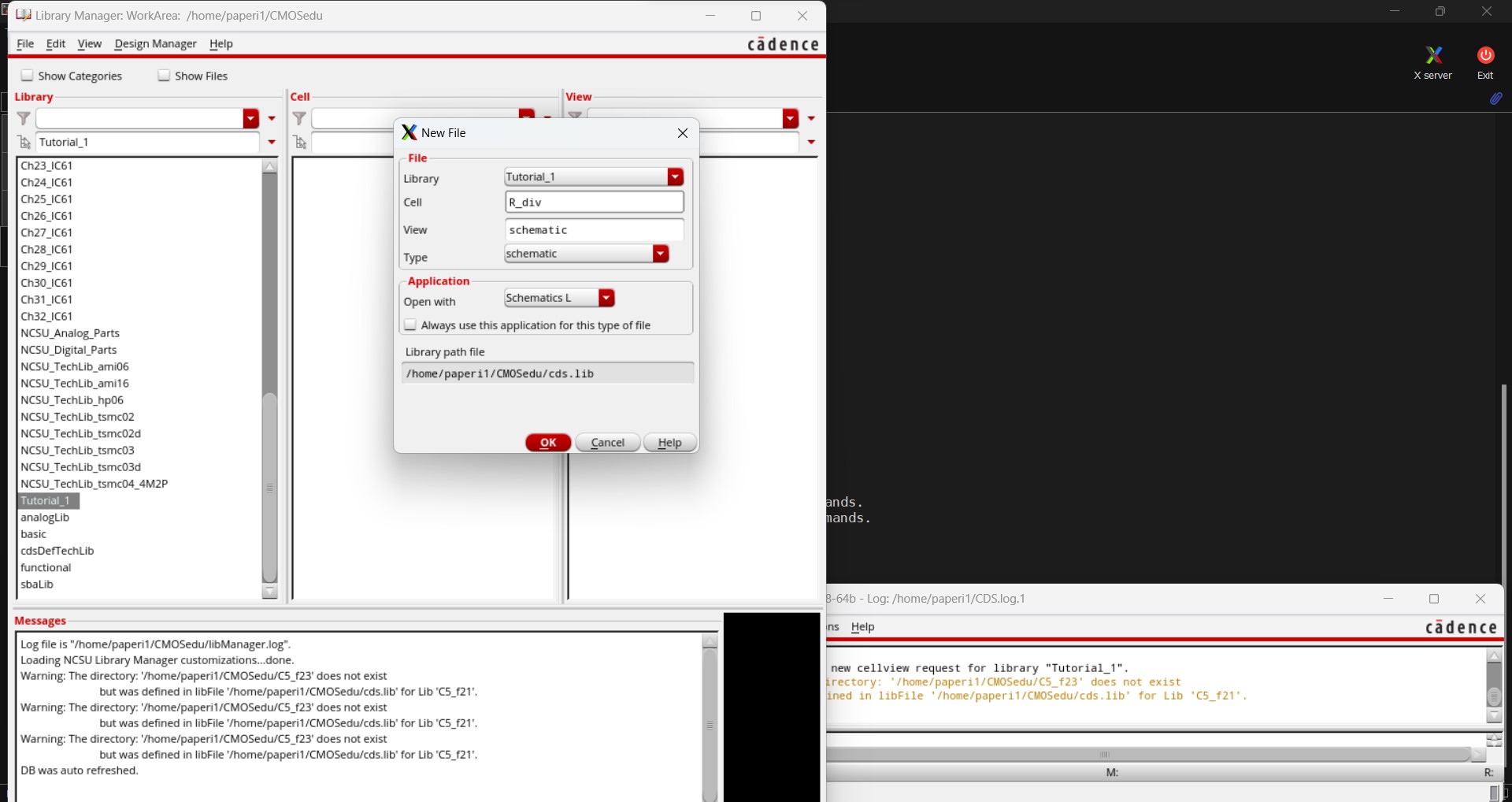
Now go back to the Library Manager and select the Tutorial_1 library that we created. Once selected go to File -> New -> Cell View and enter the information seen below. Then hit OK.

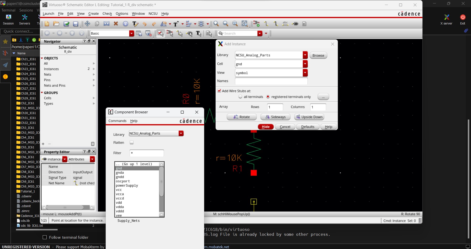
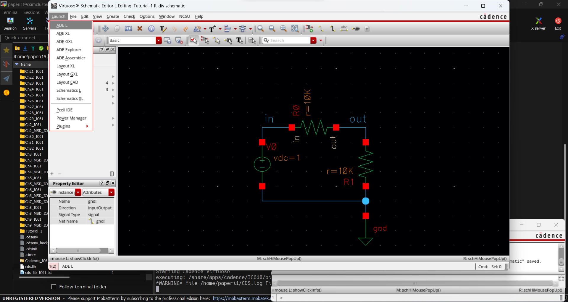
Once we hit OK a new window pops up that allows us to add components (instances) by going to Create -> Instance (or using the Bindkey I).

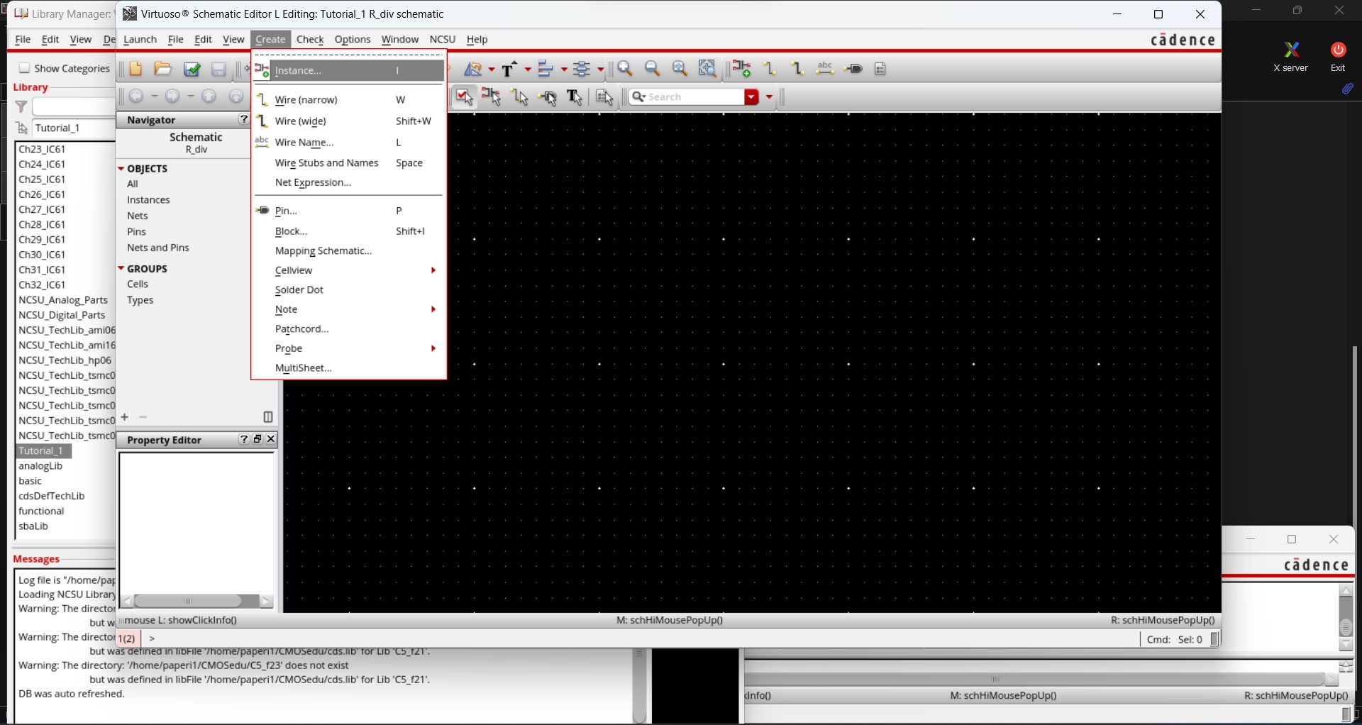
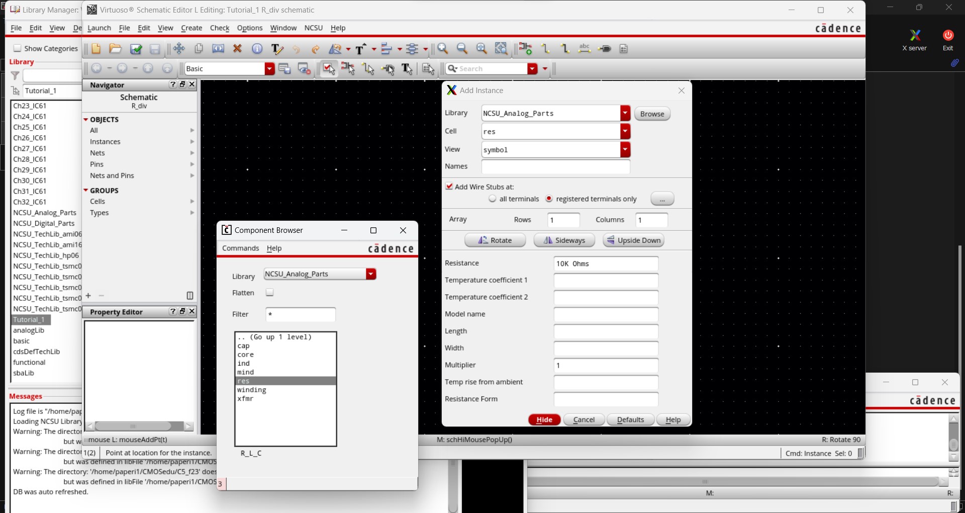
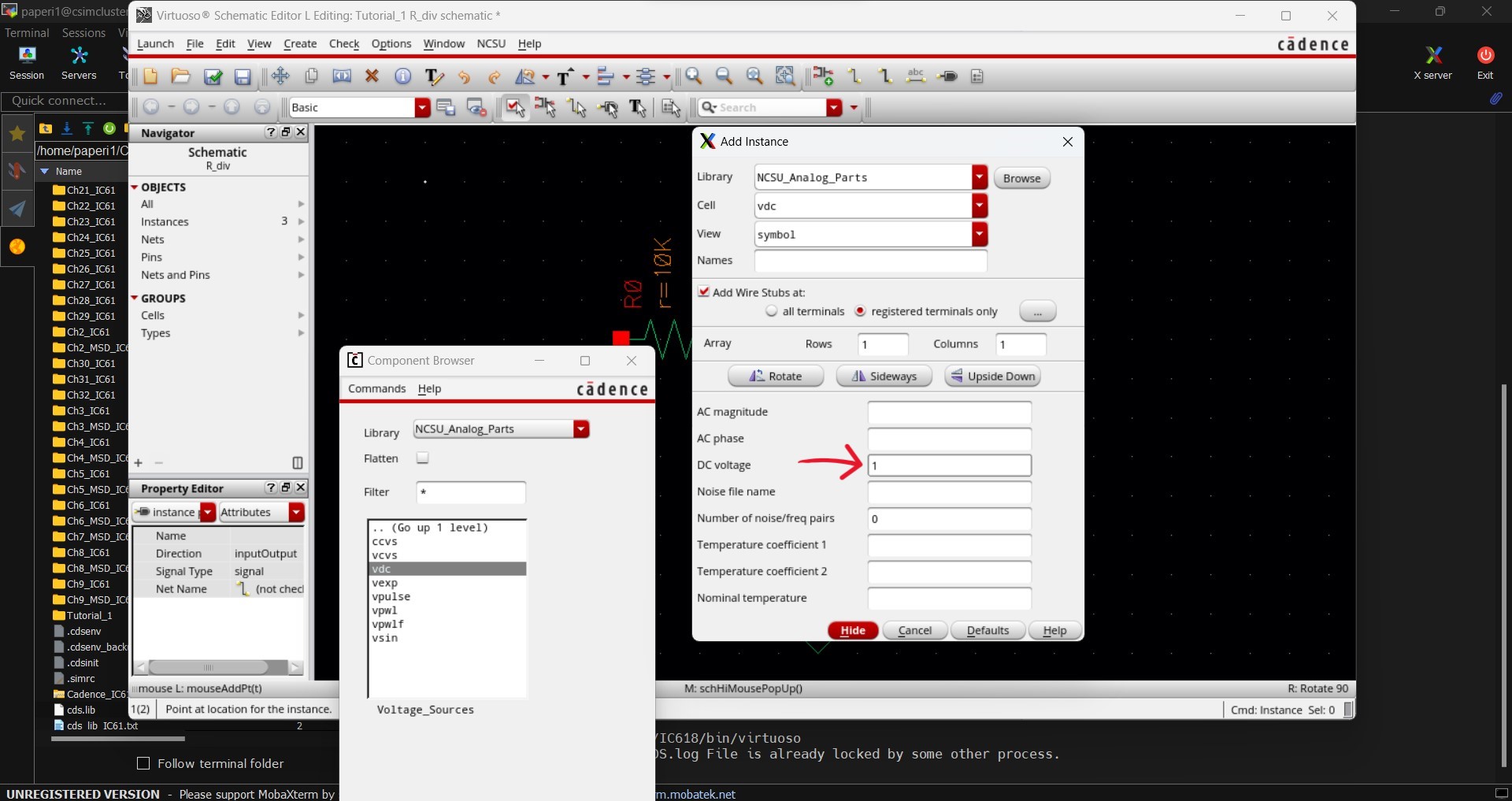
Doing so brings two new pop up menus. In the Add Instance menu we can select which library we want to use, right now we will use the NCSU_Analog_Parts library. This would automatically update the Component Browser menu to show all components within the selected library. In the Component Browser select R_L_C then res and the Add Instance menu will expand with more options. Looking back at the Add Instance menu, change the resistance value to 10k as seen below. To finish it all off, hide the Add Instance menu and minimize the Component Browser menu.

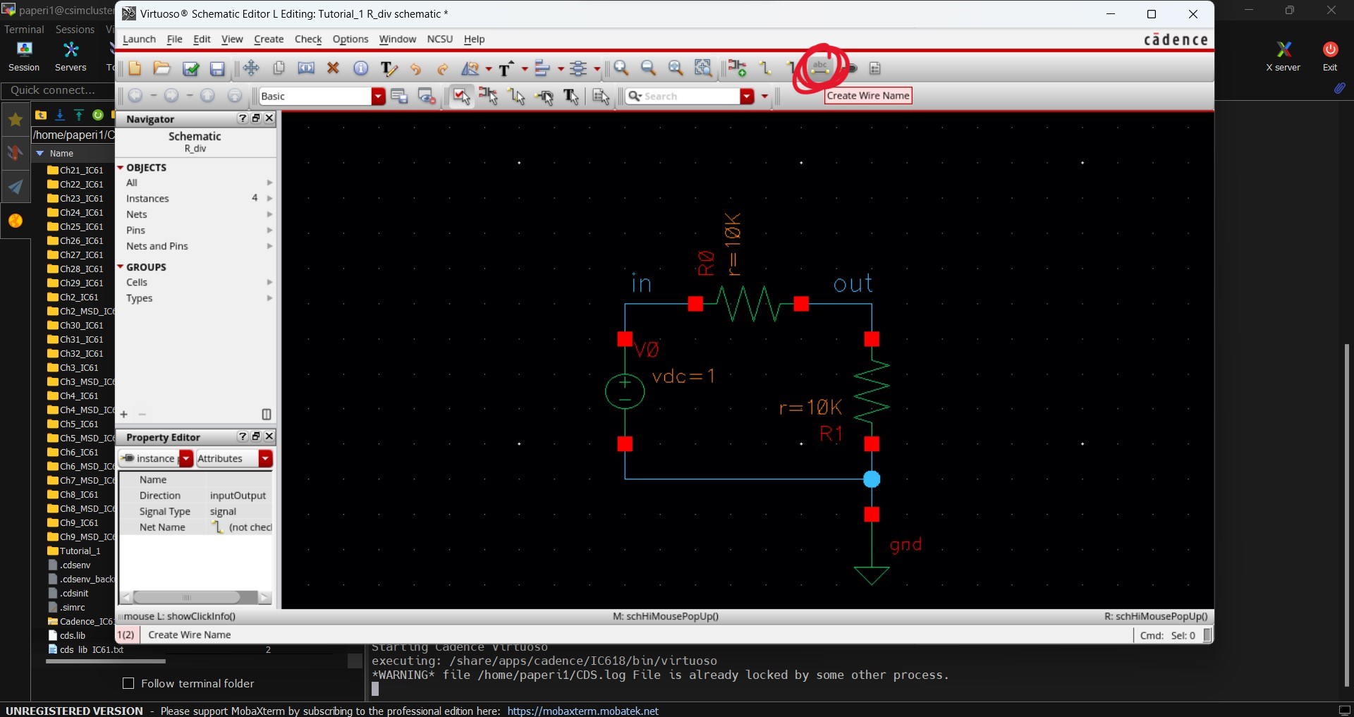
Add the two resistors as seen below. Right click the mouse (or use the Bindkey R) to rotate a symbol and press Esc to leave the Add Instance mode. To quickly fit the display, use the bindkey F. A list of all the Bindkeys can be found here.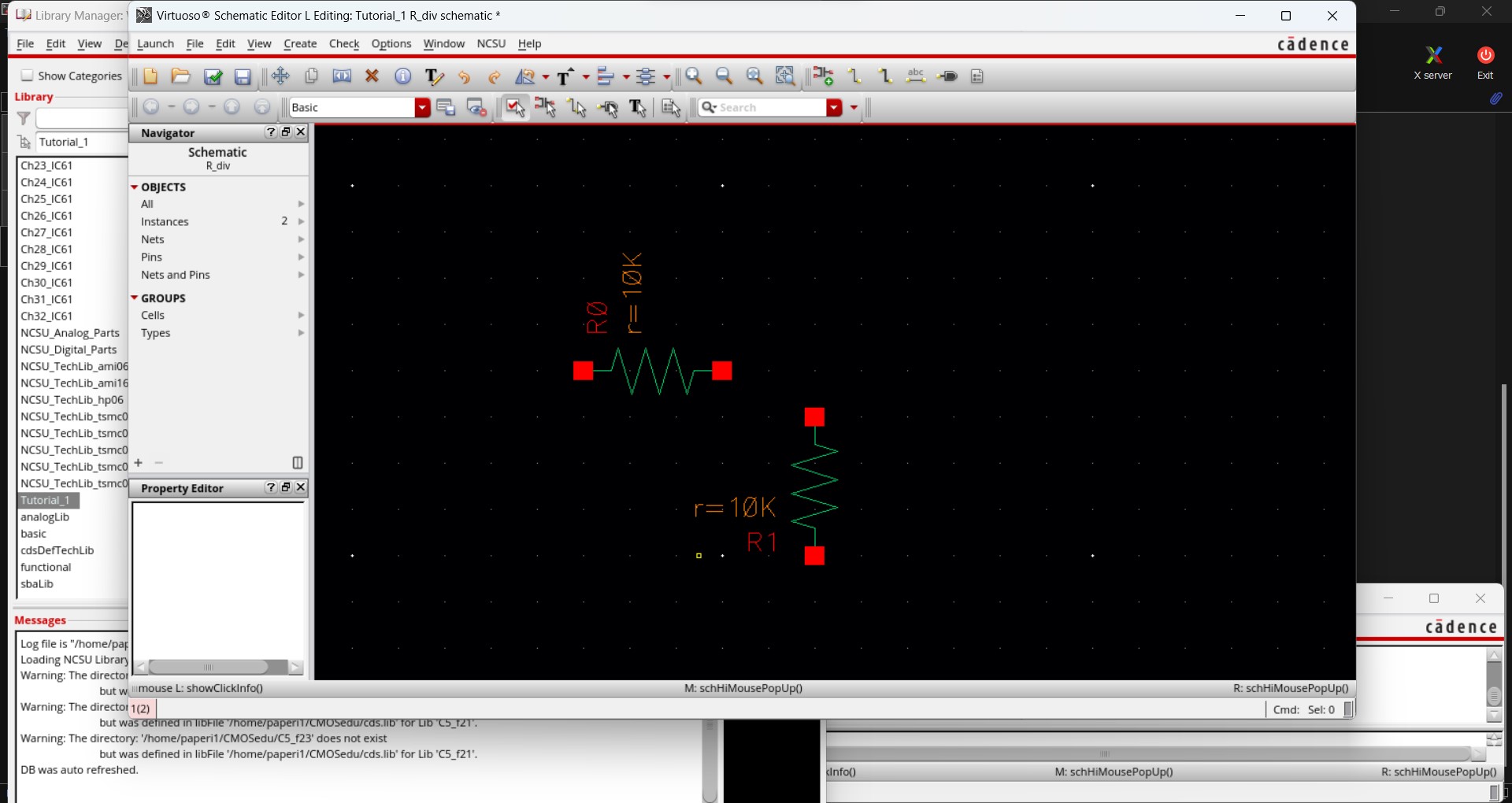

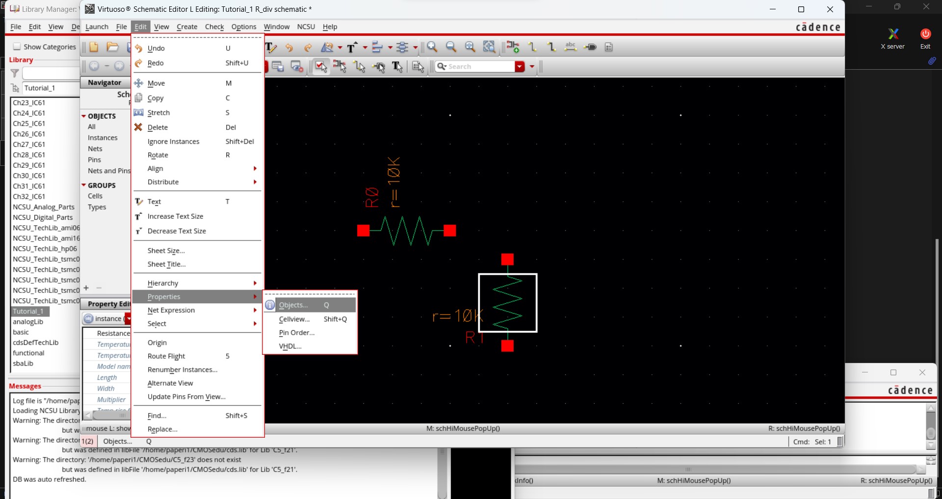
To change the resistor's value after it has already been placed, select the resistor and use Edit -> Properties -> Objects (or use the Bindkey Q). Press Esc a few times to ensure that no commands are active.

Next add ground to the schematic by pressing I (add instance), selecting Supply_Nets and gnd as seen below. If we know the name and Library of the instance we are adding, we can select them directly in the Add Instance menu without needing to use the Component Browser menu. Then use F to fit all components in the window again.

Now we'll add a 1-V DC power source. In the Component Browser menu, under Voltage_Sources, select the symbol name vdc. Then in the Add Instance menu make sure to set the DC voltage to 1V.

After placing all our symbols we need to wire them together as seen below. This can be done using the Bindkey W or the menu item circled below. 

We can lebel wires with signal names by using the bindkey L or the menu item circled below. Let's add labels as seen below.

We're almost ready to simulate the circuit now. We just need to do a "Check and Save" first. This needs to be done any time we edit the schematic, otherwise all attempts to simulate it will fail. In the Command Interpreter Window we can see if the check was successful or not, if it was not successful then we would not be able to simulate the schematic.

Now we can begin the simulation by going to Launch -> ADE L as seen below.

This will pop open a new menu, the Virtuoso Analog Design Environment (ADE). Before we simulate we need to change our simulator to Spectre (Cadence's SPICE simulator) by going to Setup -> Simulator/Direcory/Host and changing the simulator to Spectre if it is not already.

Next we need to pick our simulation analysis type by going to Analyses -> Choose. Here we will select a transient analysis (tran) with a stop time of 1 second and Enable it as seen below.

Then we need to select which signals we want to plot. To do so, go to Outputs -> To Be Plotted -> Select On Schematic.

From here, go to your schematic and select the wires as seen below.

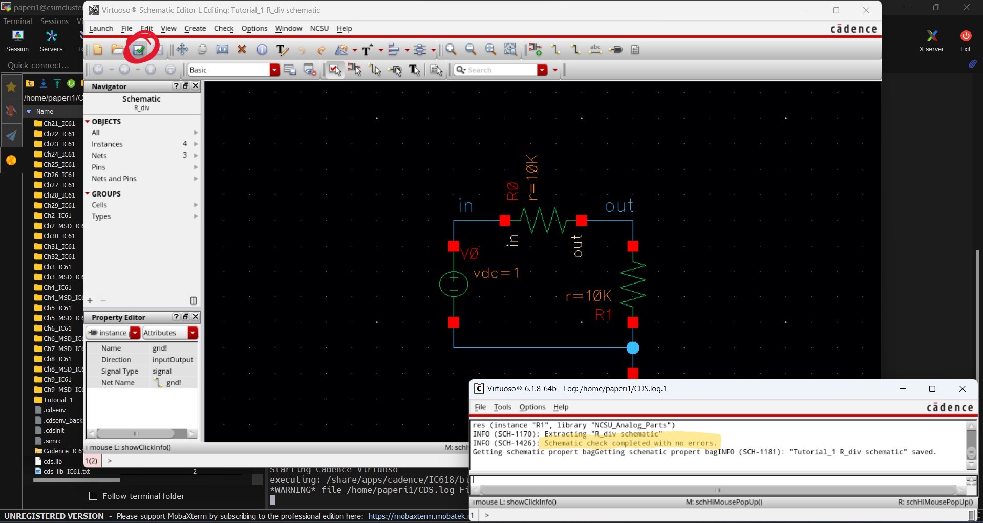
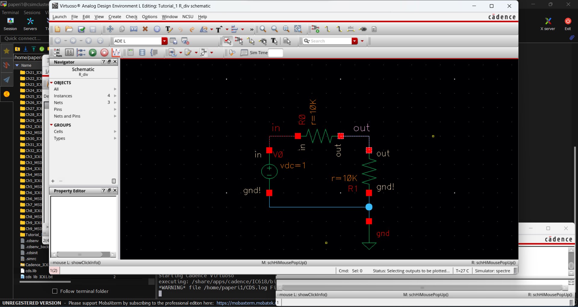
Looking back at the ADE, we should see the following.

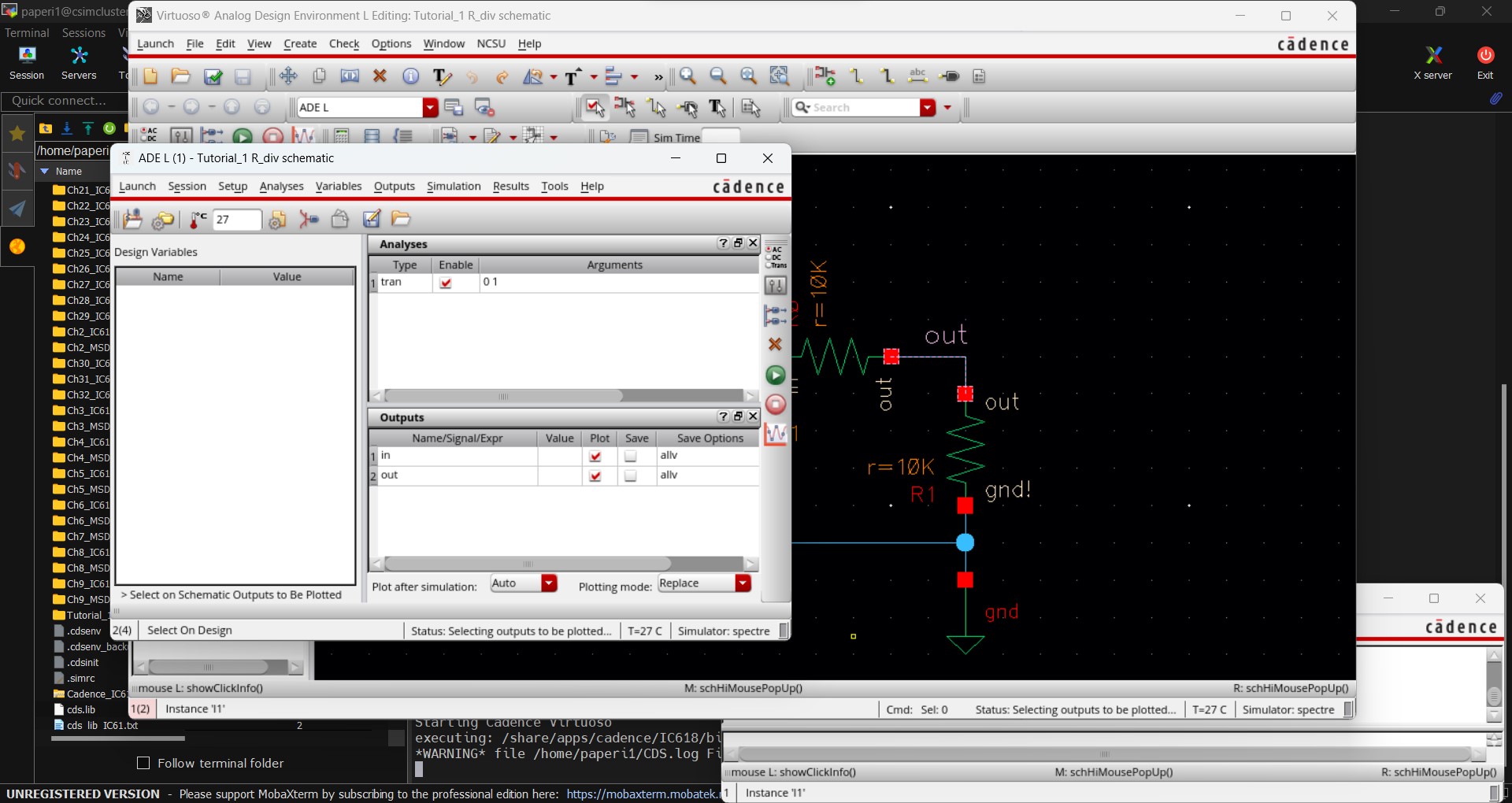
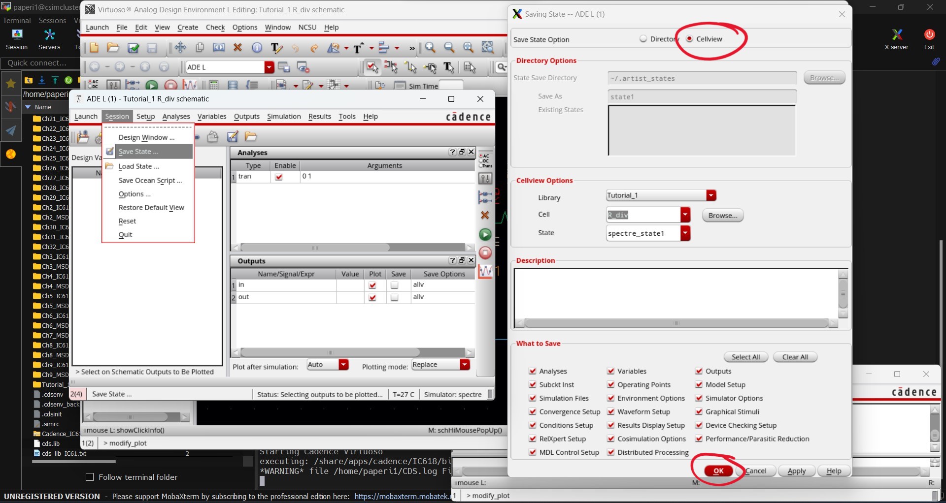
We are finally ready to simulate the circuit and can do so by pressing the green "Netlist and Run" button. However, before we run the simulation it is best to save this information so future simulations of this circuit would not need to go through all these steps again. In the ADE menu go to Session -> Save State and select Cellview then hit OK.

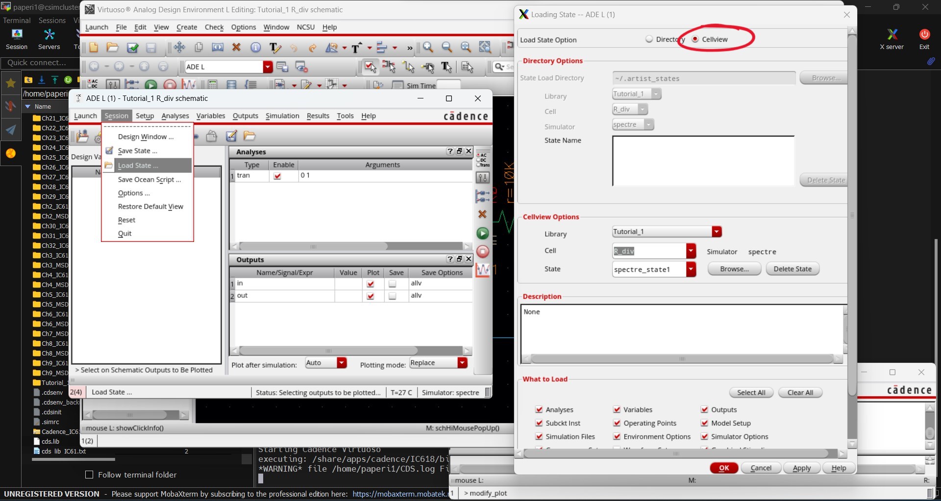
To load this state we would select, in the ADE menu, Session -> Load State and make sure to select Cellview then OK.

Finally we can hit the green play button and run the simulation to get the following results.

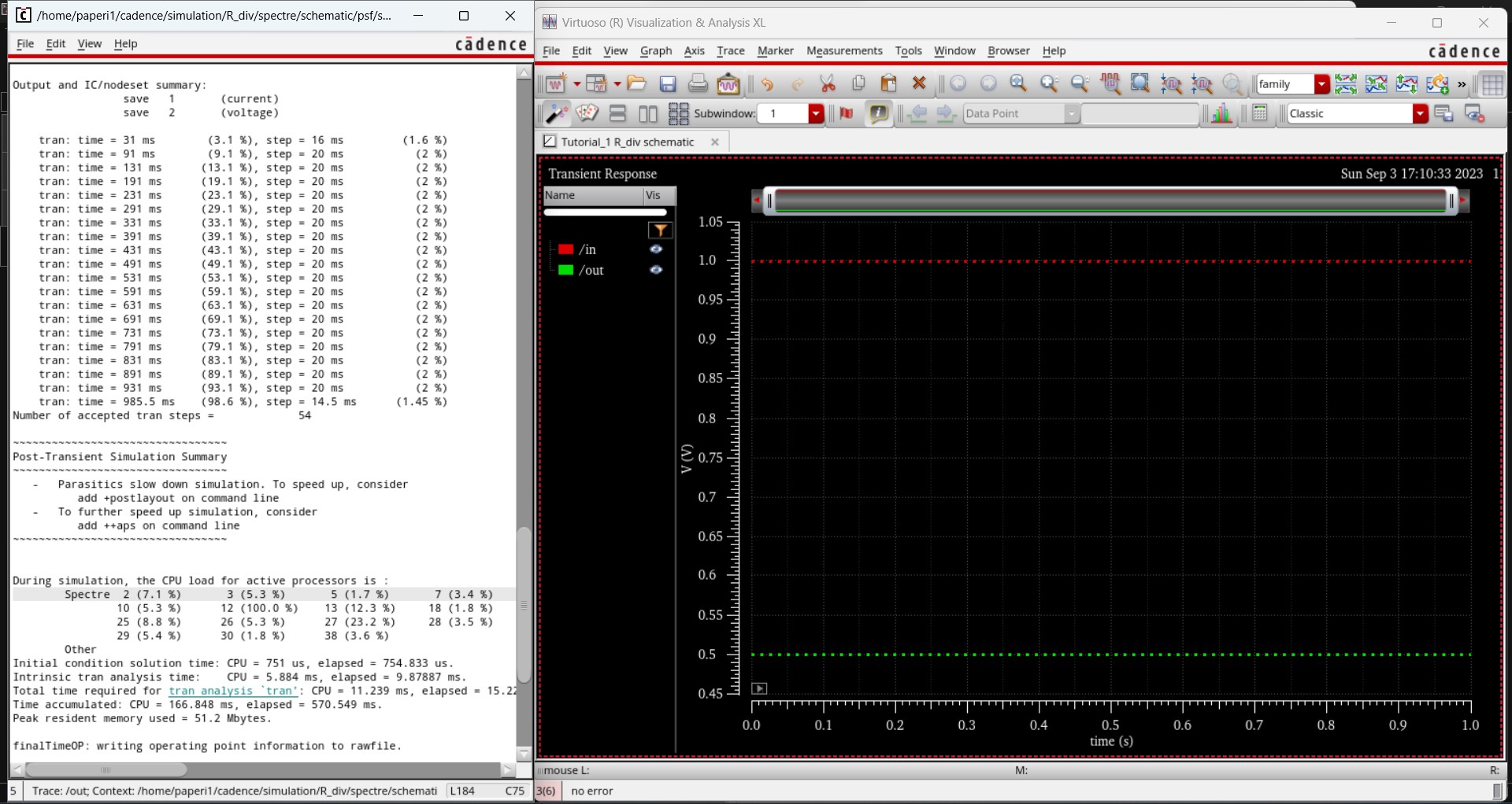
This concludes the portion of Tutorial 1 that we are meant to cover.

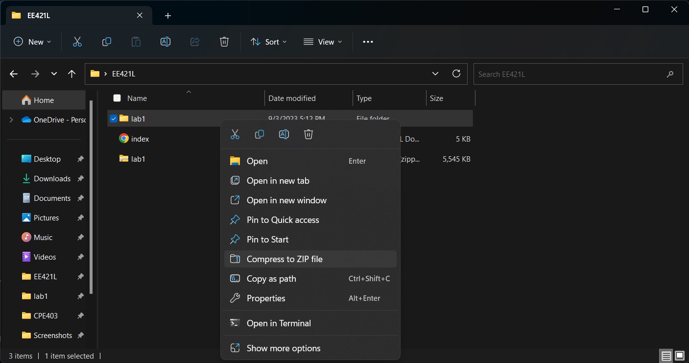
Throughout this lab, and all future labs, I have contsantly backed up my lab after every couple steps. To ensure the most accurate protection, I have backed up my lab work by zipping it all up and sharing it with myself in two different ways.

First off, I have all my work saved to my desktop before even attempting to upload it to the CMOS website. After every couple steps I zip up everything in my lab folder and save it to my desktop.

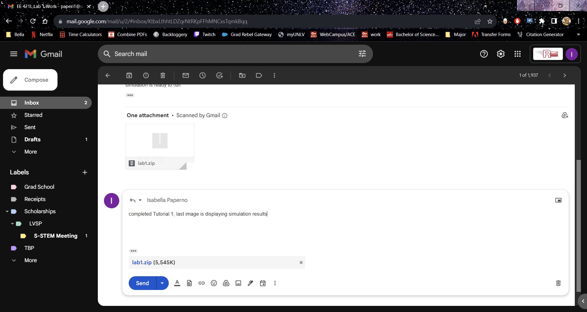
Once all my work is zipped up I open up my UNLV email and send it to myself with a breif update on what steps have been completed since the last backup.

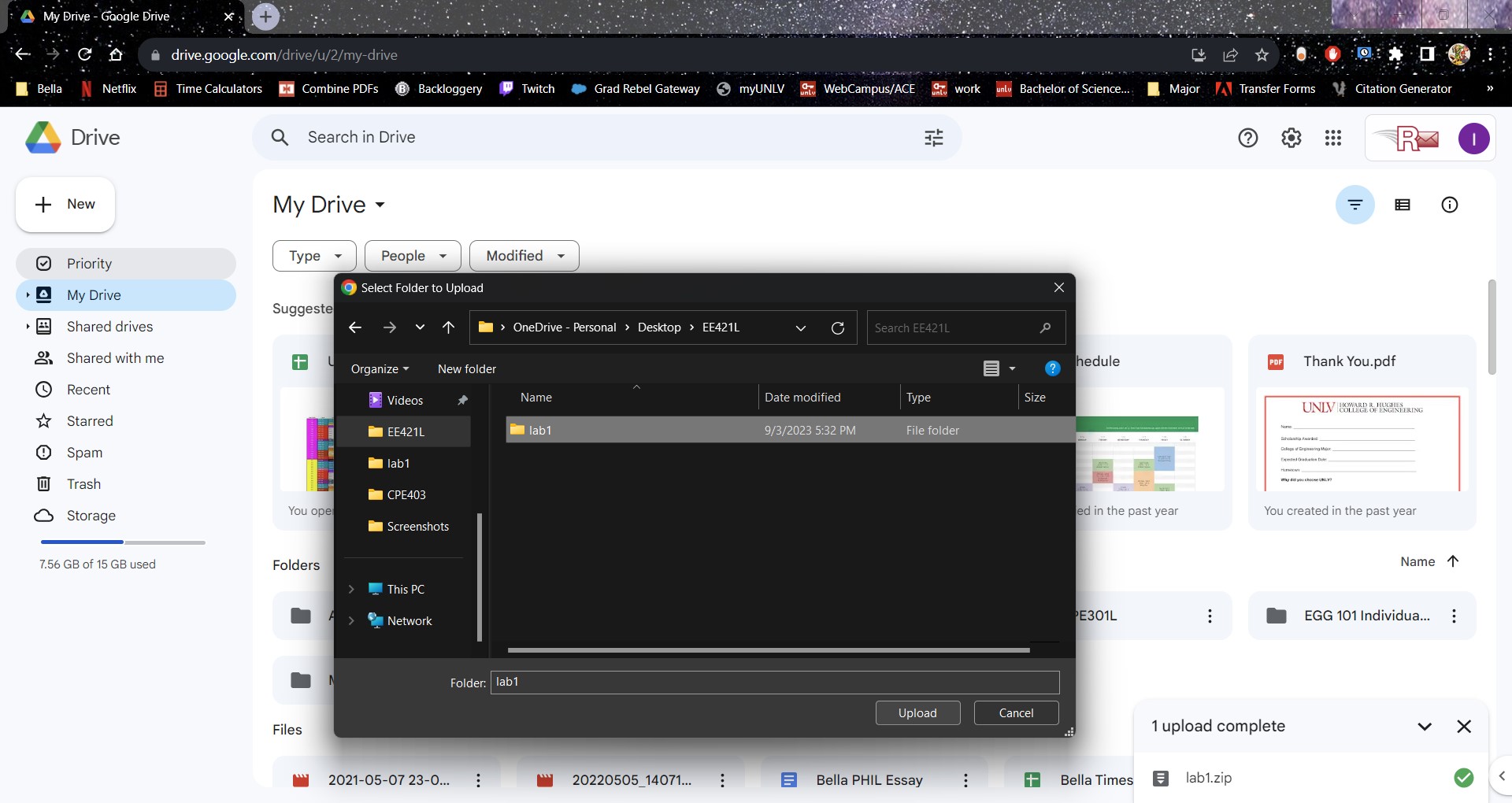
Finally, just to be safe, I also upload both my zipped lab work and all lab work in my desktop folder to my Google Drive.

Return to EE421L Lab listings