Lab 1 - ECE 421L 

Authored by Kyle Abenojar, abenok1@unlv.nevada.edu

September 6th, 2023

Prelab:

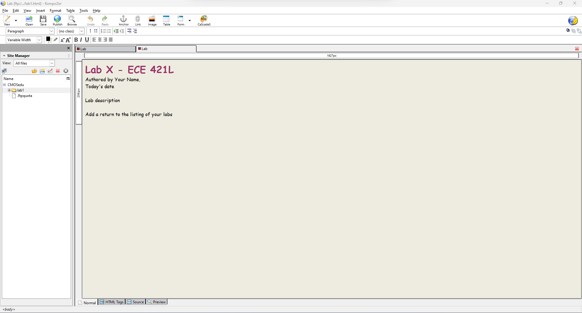
For this lab, we had to make our CMOSedu accounts, and get familiar with logging in and editing webpages using KompoZer.

After receiving my CMOSedu account login, I was able to log in via file explorer and access my folders on the cmosedu webpage. Here, I am able to create folders and upload files to generate my lab reports. 

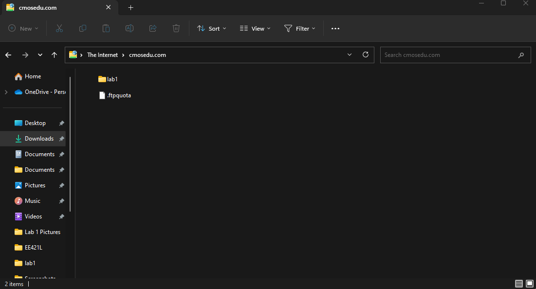
The lab reports will be drafted using html which can be edited using the KompoZer program. After making the report, I can then publish the report as a webpage on cmosedu.com.

Lab Report:

Lab Description: This lab serves as an introduction to the various tools that we will be using throughout the semester: KompoZer, Cadence, MobaXterm etc. In this lab, we will set up and become familiar with performing simulations in Cadence, learn how to generate and submit our lab reports using KompoZer and file explorer, and ensure we perform proper practices to protect our work by backing up our data. 

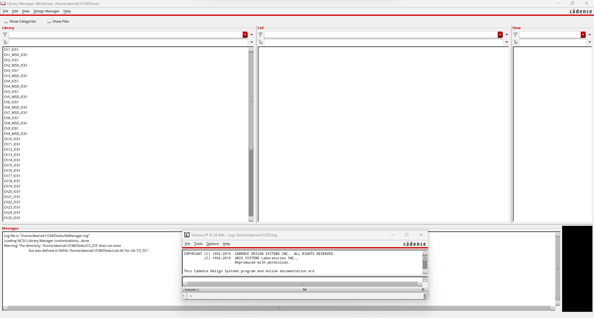
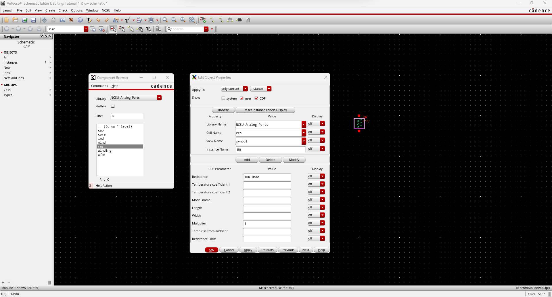
After logging into the UNLV servers using MobaXterm, we are able to launch virtuoso by typing the command "virtuoso &" into the terminal. Subsequently, the Command Interpreter Window as well as the Library Manager Windows open as pictured below.

We then generated a new library by navigating in the File Tab in the Library Manager. We named the new library Tutorial_1.

After generating the new library, we looked in the cds.lib file located in our CMOSedu file to see what changes were made. Here we see that the line "DEFINE Tutorial_1 /home/abenok1/CMOSedu/Tutorial_1" was added to the bottom of the text file. This tells Virtuoso where to look for the files in the Tutorial_1 library.

By hitting the I key on our keyboard, we pull up the component browser. By navigating to the proper folders, we pull up a resistor and place it on the schematic and give it a resistance of 10k Ohms.

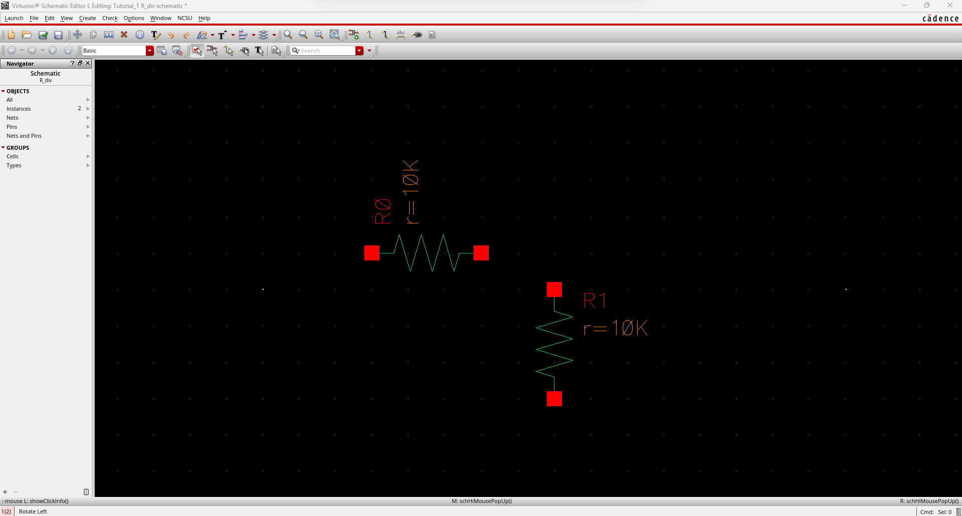
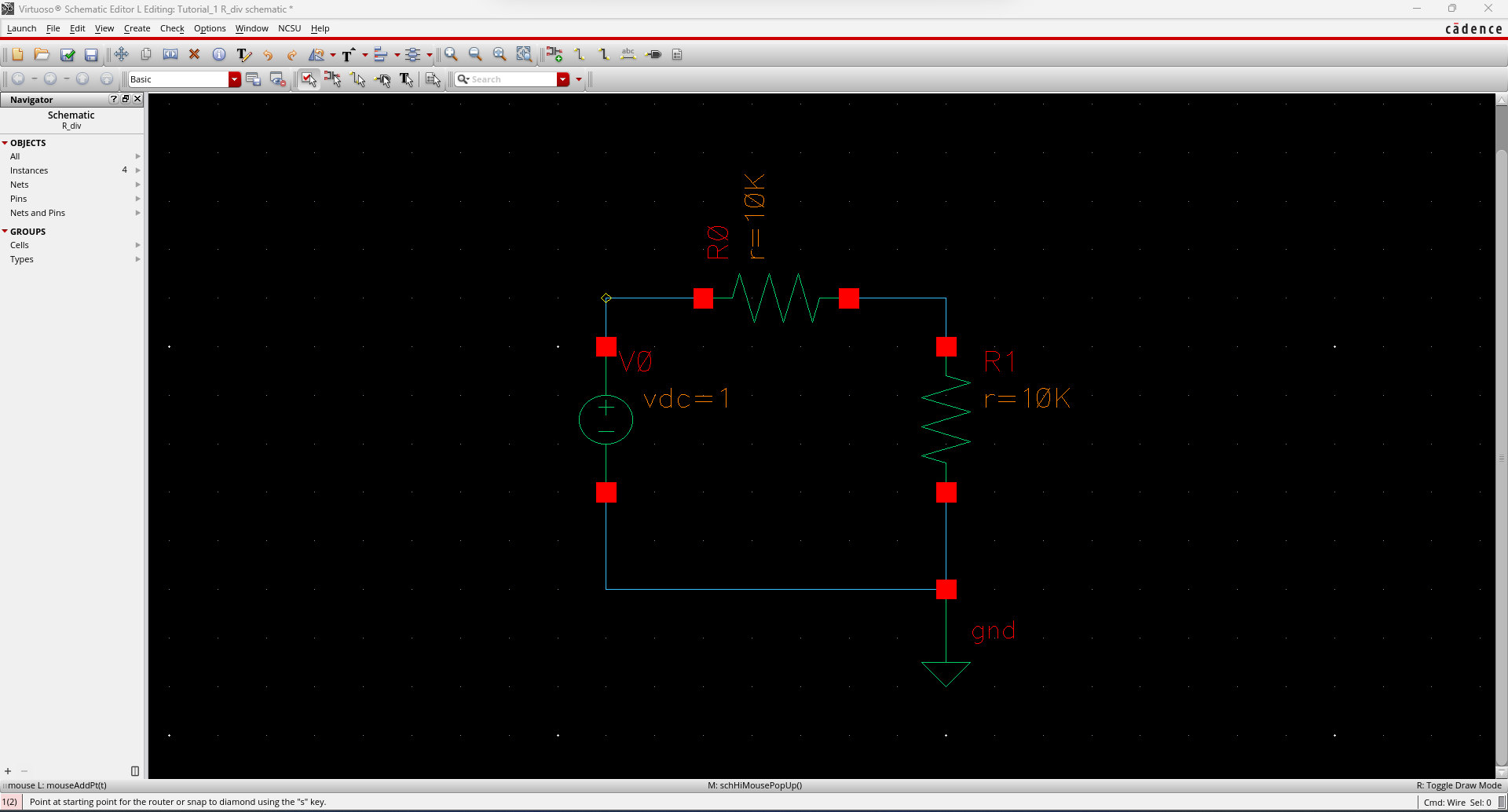
By hitting the C key, I was able to copy and paste a second 10k resistor on my schematic.

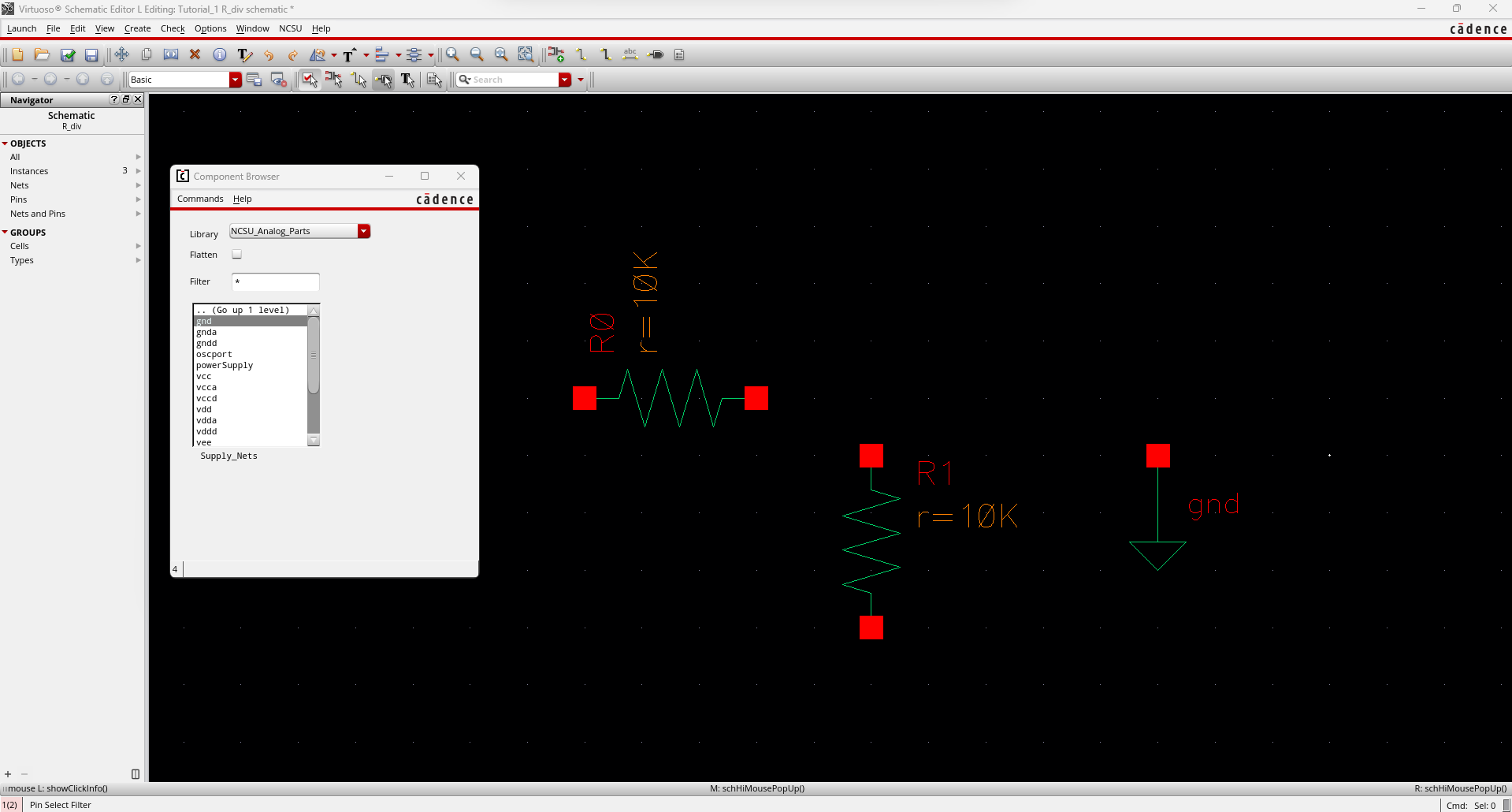
By pressing the I key once again, I pull up the component browser and generate a ground.

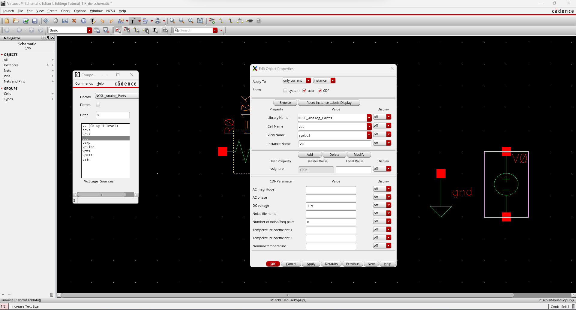
We pull up the component browser one more time to generate a DC voltage source. We are able to change the properties of the voltage source by clicking on the component and pressing the Q key. This allows us to set the voltage to 1V.

By using the M key, we are able to move the components around the schematic. Then, by pressing the W key, we can wire the components together. Lastly, by pressing the F key, we can get a full view of our circuit.

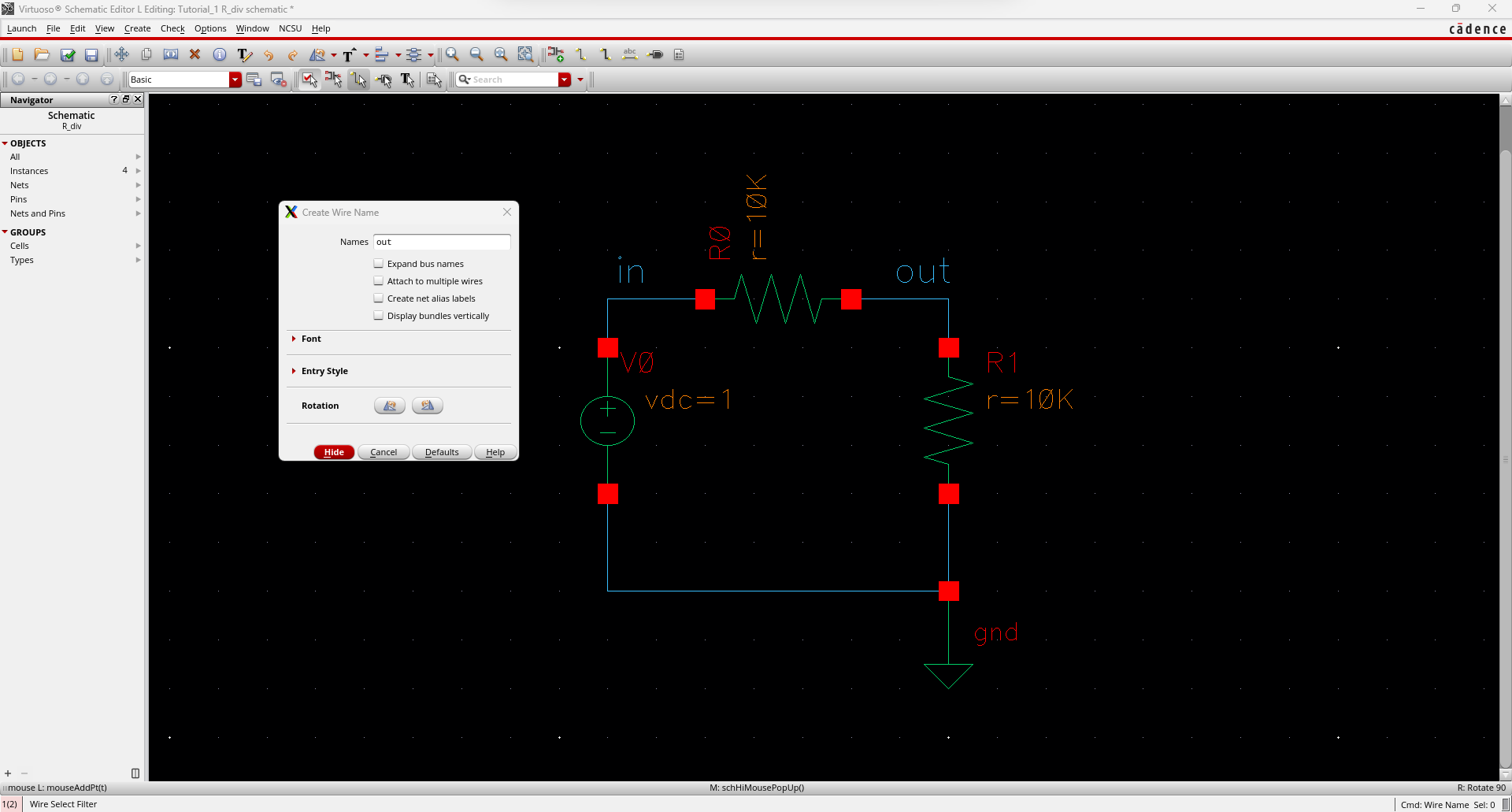
By clicking on the label button, we are able to generate labels and name the wires in our circuit. Here, I named the node after V0, "in" and I named the node after R0, "out".

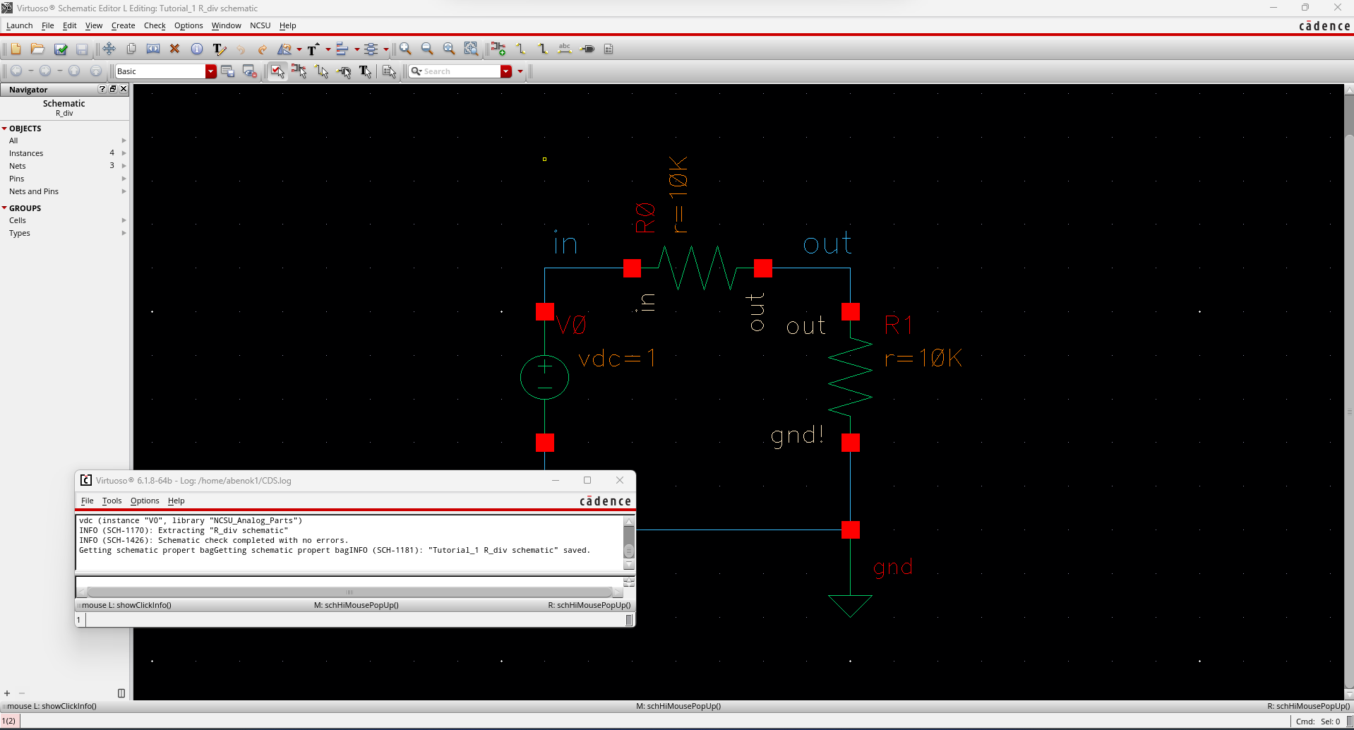
Before simulating, we must click the check and save button. If there are no errors, this will be indicated in the command interpretor window.

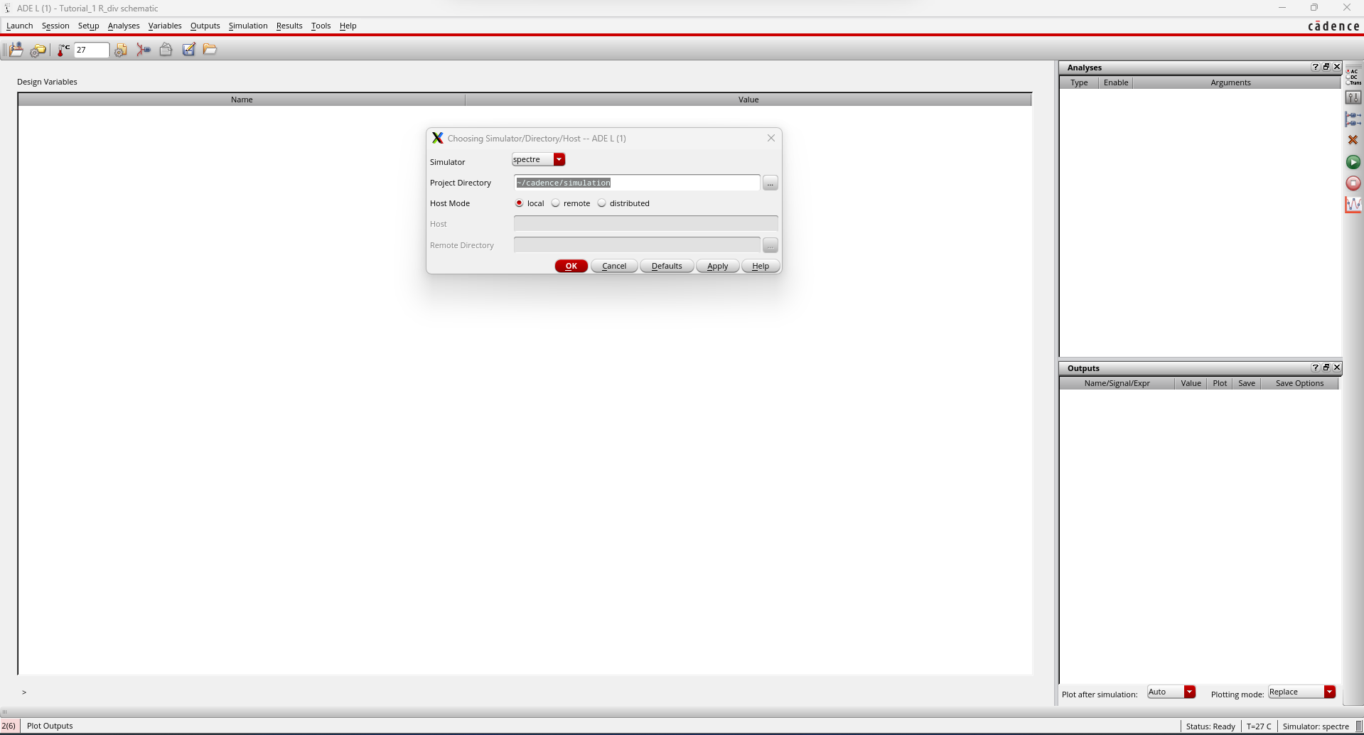
By clicking on the launch tab and clicking on ADE L, we are able to launch the Analog Design Environment window.

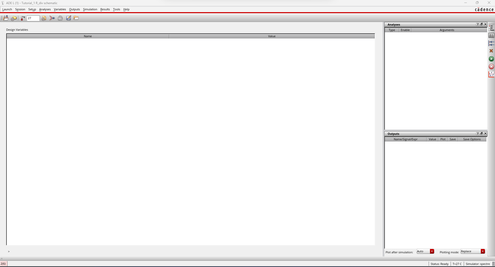
In the Setup tab, we click on the simulator button to ensure that our simulator is set to spectre.

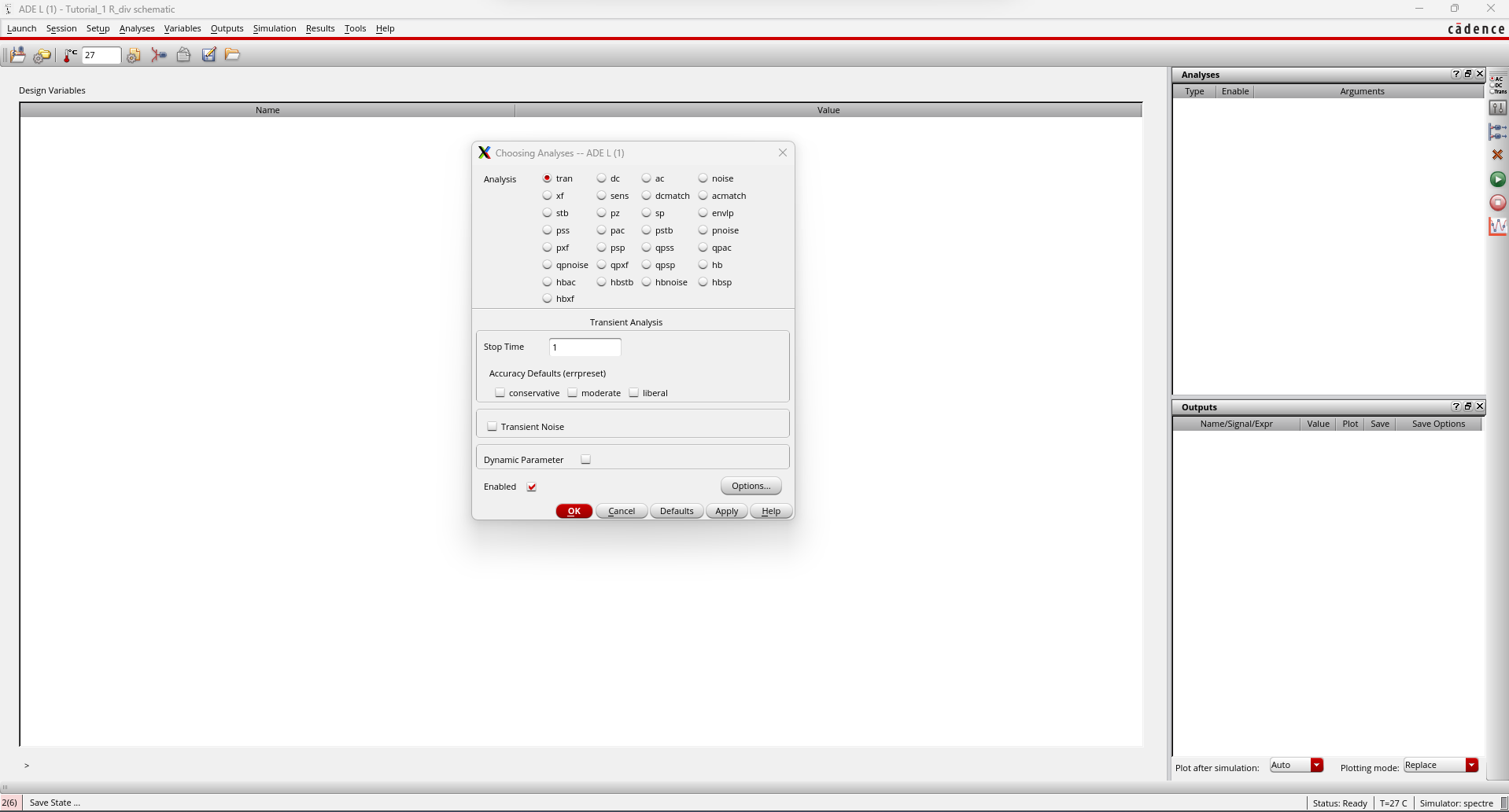
Next, we must choose the analysis we want the tool to perform. We click on the analysis tab then click choose. This brings up the following menu. In this case, we want to perform atransient analysis.

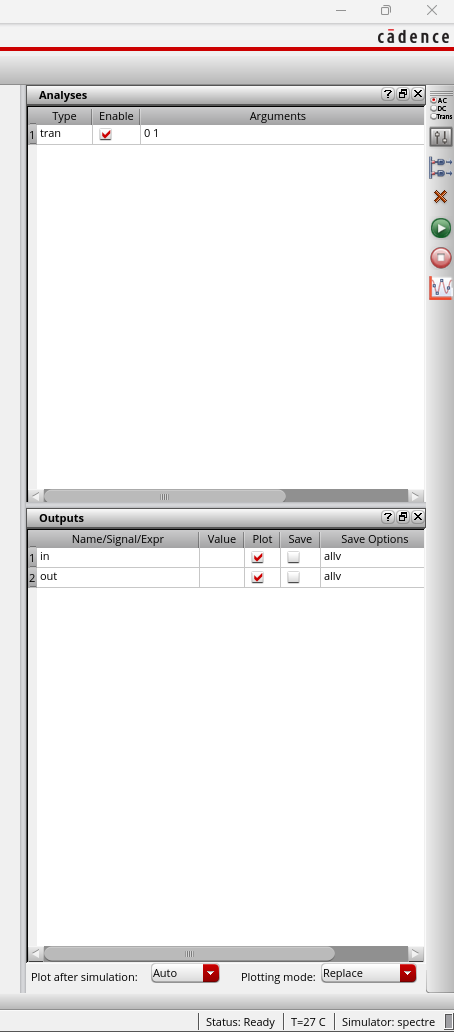
After choosing our analysis of choice, we can choose our outputs but clicking on the outputs tab, then clicking on to be plotted and lastly select on design. I chose the nodes I labeled in and out. I knew I did this correctly because in my the ADE window, I can see that in and out have been labeled as outputs.

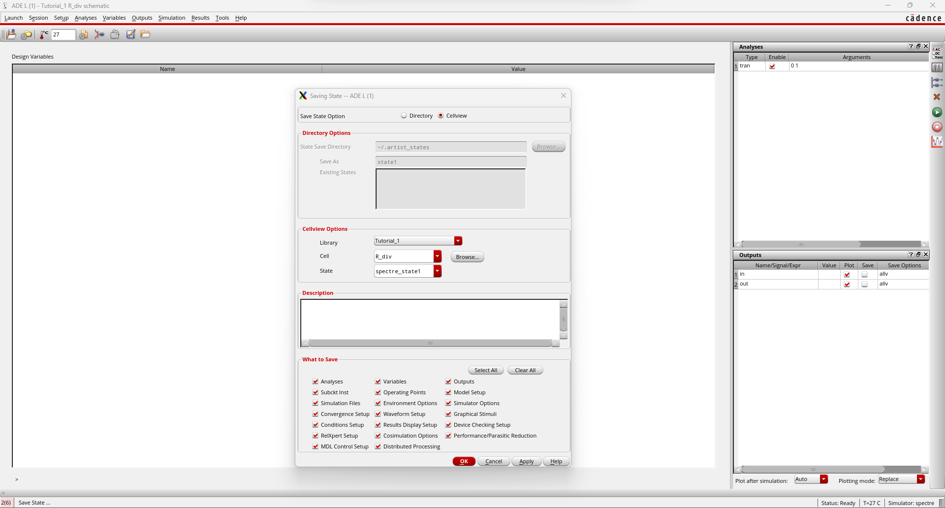
In order to save us time in the future if we were to reuse this simulation, we save the state of the simulation so that we can simply load it up again.

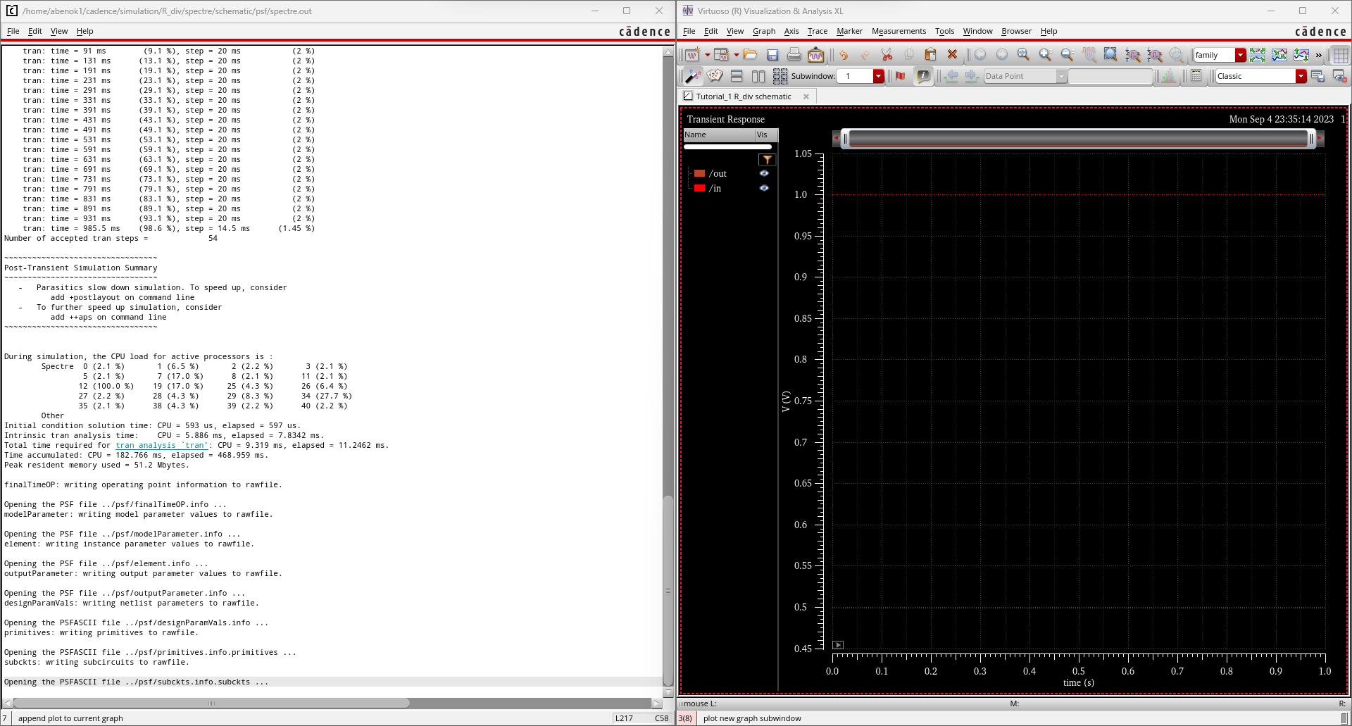
After this, we click on the green play button on the right of the ADE window. The window on the left of the picture below pops up first indicating that thee plot is being generated. Once the simulation is done, the plot on the right appears.

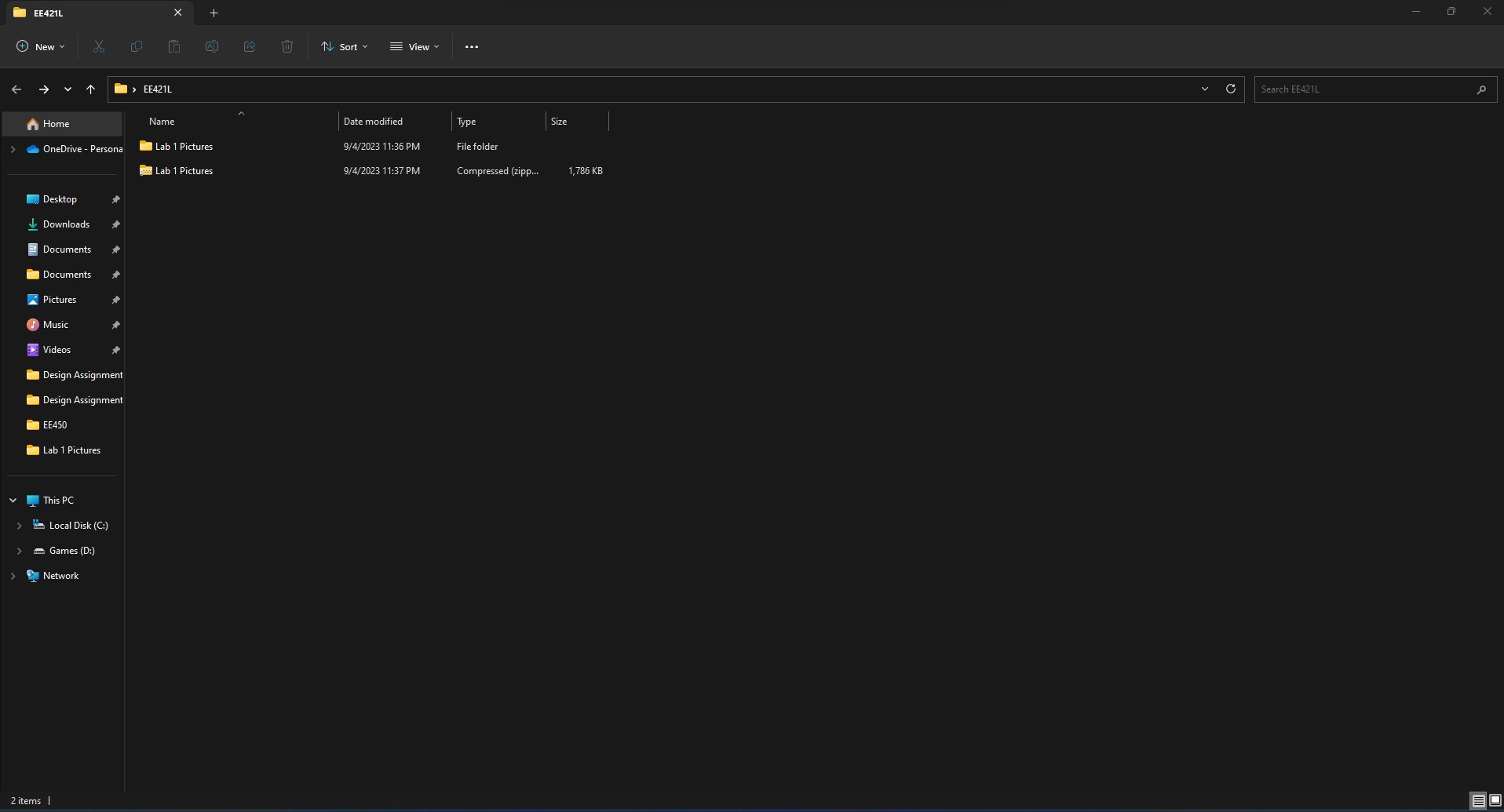
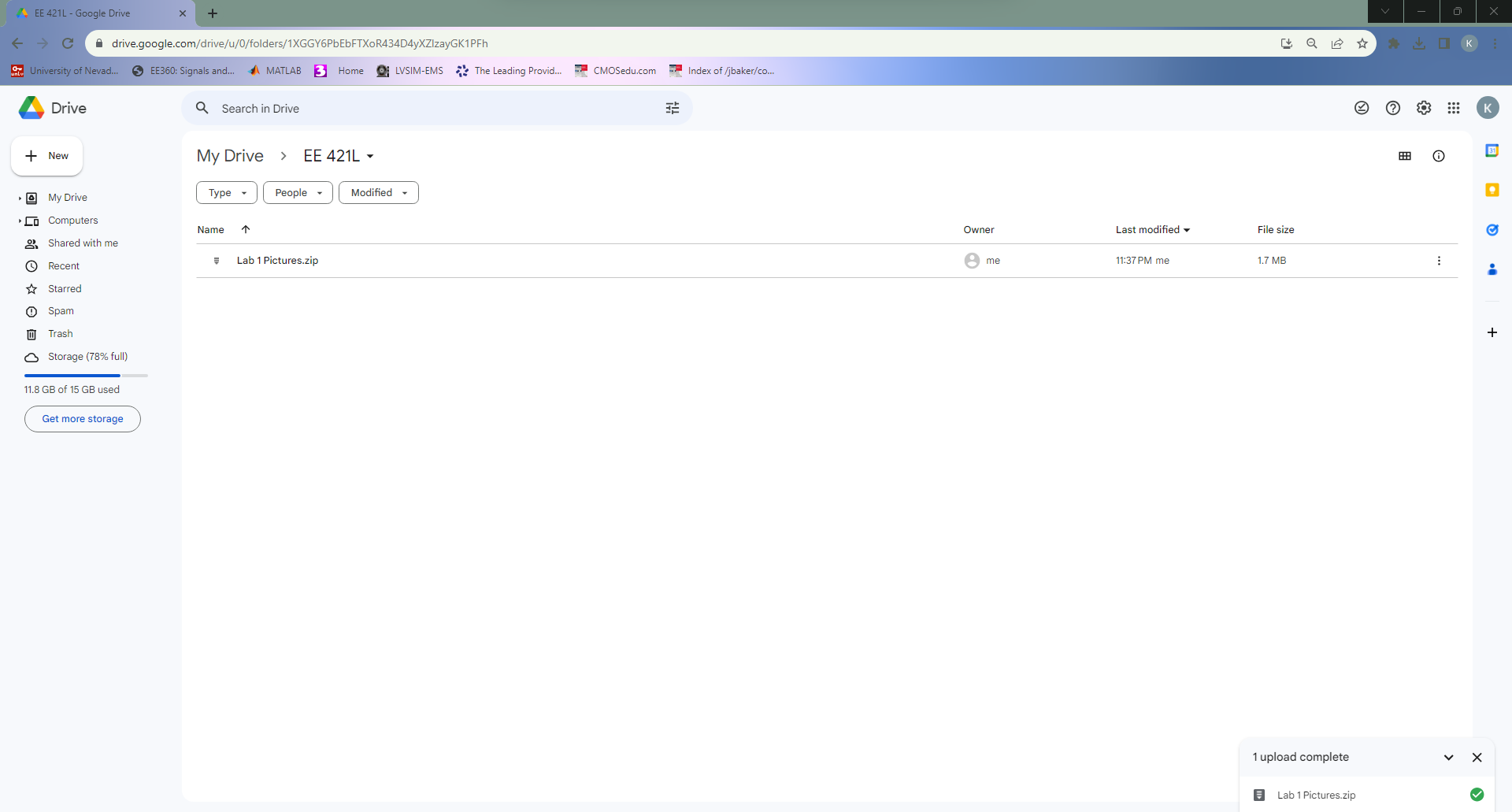
It is important to save our work and create backups. Here, I show a local copy of a folder containing all of the pictures I generated for this lab. I then zipped this folder to upload a back up online.

My storage of choice is my Google Drive account. Shown below is my zip file containing all my pictures uploaded to my Google Drive.

Return to 421L Labs