Lab 4 – Op-Amps II: Gain-Bandwidth Product & Slewing
EE 420L Analog IC Design
Lab Date: 2/20/19 Due: 2/27/19
Last Edited on
2/20/19 at 9:58pm using Word
Suppose we
have an Operational Amplifier (Op-Amp) and we would like to operate the Op-Amp
at different frequencies. Ideally, we can tell ourselves that we can get any
Gain at any frequency that we want, however,
the world is not perfect and there will be some drawbacks for wanting to
have high-speed circuits. All of these gains will all “roll-off” and unify at
one given point at dB = 0 (gain of 1), and this point is called the Unity Gain Frequency. The roll-off
point for higher gains is called the Bandwidth.
-Also, suppose
we want to send some very fast pulse through an amplifier. We will also realize
that there are device limits set so that we can have a certain volt gain per
certain time. This certain parameter on the device that will give us this limit
is called the Slew Rate.
In this lab,
we will be figuring out the bandwidth frequency (or f3DB or roll-off
frequency) for both the Non-inverting and Inverting Op-Amp topology. Also, we
will build a simple circuit so that we can find the point where the Op-Amp’s
output will show its slew rate for both a square wave and a sine wave.
--------------------------------------------------------
Experiment
1: Non-inverting Op-Amp
In this
experiment, we will build the non-inverting op-amp and testing out gains of 1,
5, and 10 and finding the Bandwidth frequencies of these gains, respectively.
Before we do
these experiments, we will need to prove these bandwidth frequencies using 2
methods:
Method A. Hand Calcs:
To solve for
this bandwidth frequency, we will need a simple equation to solve for our
frequencies.
The
Gain-Bandwidth equation will be given by:
Gain * Bandwidth = Open Loop
Gain (constant)
So, given a
gain of 1 V/V and knowing the Bandwidth, We can say
that:
| 1 V/V | * 1.3MHz = 1.3M Open
loop gain.
Theoretically,
our bandwidth for a gain of 1 should be 1.3MHz.
For a gain of
5 V/V: AoL / Gain =Bandwidth
= 1.3M / 5 =
260kHz
For a gain of
10 V/V: 1.3M / 10 = 130kHz
Method B. Looking at the Open
Loop Gain Graph:
Suppose we are
here to look for quick numbers and do not have access to our calculators. The
datasheet will provide us with a graph and we can use this graph to estimate
what our bandwidth will be for any given closed loop gain.
Here is a
graph giving us our Open Loop Frequency Response, found in the LM324.pdf datasheet:
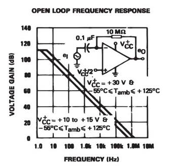
So using our
eyes, we can see that:
For a gain of
1: For
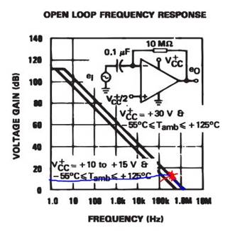
a gain of 5:
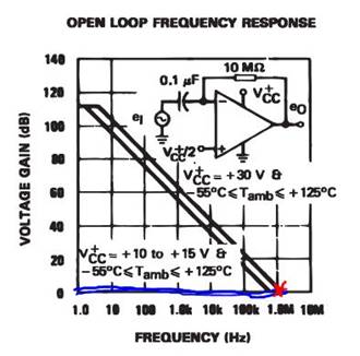
Bandwidth = 1.3MHz
Bandwidth = ~300kHz
For a gain of
10:
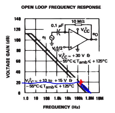
Bandwidth = ~150kHz
Here is a
table recapping all of the hand-calculated Gains
|
Gain |
1 V/V |
5 V/V |
10 V/V |
|
Bandwidth |
1.3MHz |
260kHz |
130kHz |
Experiments:
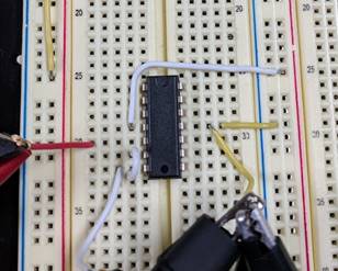
For a gain of 1,
we will be building what is called a Unity-Gain Amplifier, which is the
Non-Inverting Op-amp topology but the output is fed back into the inverting
terminal of the op-amp.
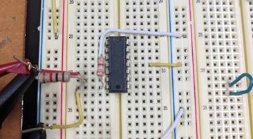
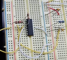
On the breadboard:
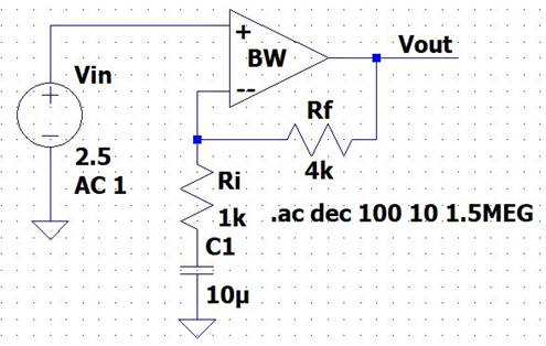
LTSpice Schematic:
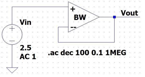
The op-amp’s VCC+
and VCC- are 5V to 0V, respectively. The input will be a 1Vpp, 2.5V DC offset.
To find this
bandwidth frequency, we will be looking for when our output is 70.7% of the
input.
NOTE: .707 comes from doing 1 / sqrt(2),
where both our real and imaginary parts are equal to 1.
Bandwidth for Gain of 1:
Here we can
see that we will get this bandwidth frequency at:
Bandwidth = around 1.3MHz
To simulate this
Roll-off in LTSpice, we will do a simple calculation:
Since we will
want a Low-pass bandwidth, we will do this circuit inside our Op-amp circuit:
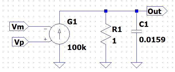
For the capacitor,
we will use the RC time constant. From the datasheet, at a low frequency of
10Hz, and given a resistance of 1 ohm, f3dB = 1 / (2πRC) =>
Capacitor = 1 / (2π(1)(10Hz)) = 0.0159 Farads
Here is our LTSpice Gain of 1 output:
As you can
see, the 3dB value will be at around 1MHz. The reason for this inaccuracy is
that we have created our own ideal Op-Amp, but we want to estimate and try to
simulate what it will look like on the board.
Gain of 5:
For a gain of
5, we will be using RF = 4kΩ and RI = 1kΩ so
that our Non-Inverting gain will be:
ACL
= | 1 + (4/1) | = 5 V/V
On The breadboard:
NOTE: RI’s Terminals are
connected to a 2.5V DC battery source and to the Inverting Terminal.
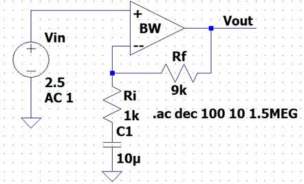
LTSpice:
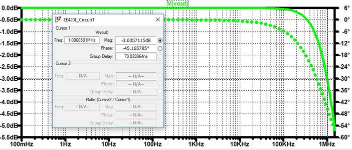
Output:
NOTE: 100mVpp*5/2 *(.707)=
176mV
The point that
we get to see that the Output rolls off to 70.7% of the input is at
Bandwidth = 190kHz
LTSpice Output:
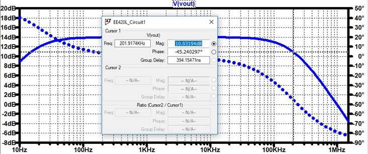
From here, we
have our top dB of 14dB and subtracted 3dB to get 11dB. F = 202KHz
Gain of 10:
We will swap
out RF = 9k and RI = 1k so that we will get a gain of 10.
LTSpice:
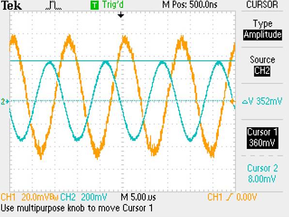
Output:
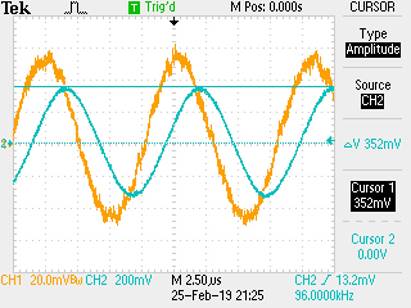
NOTE: 100mV*10/2 * (.707) = 352mV
Bandwidth = 96kHz
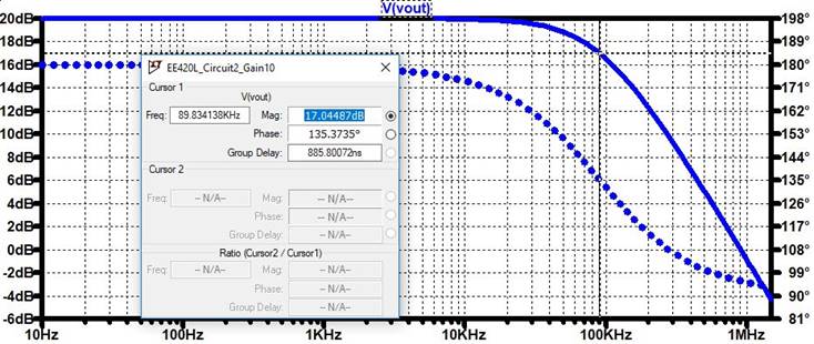
LTSpice Output:
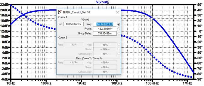
20dB – 3dB = 17dB,
Bandwidth = 100kHz.
|
1 V/V |
5 V/V |
10 V/V |
|
|
Experimental |
~1.3MHz |
190kHz |
96kHz |
|
Hand Calc |
1.3MHz |
260kHz |
130kHz |
|
LTSpice (Ideal) |
1MHz |
202kHz |
100kHz |
From the table,
we can conclude that our hand calcs are in the ballpark on where our
experimental bandwidths are. For LTSpice, it was used
as a reference to estimate where the roll-off frequency is.
----------------------------------------------------------------------------------------------------
Experiment 2: Inverting Op-Amp
For this
experiment, we will do what we did in experiment 1 but for the inverting op-amp
topology.
For this, we
will use our simple equation:
Gain * Bandwidth = Open Loop
Gain (constant)
| 1 + Rf/Ri | * Bandwidth = AoL
Then to find
the Gain-Bandwidth Product:
| Inverting gain | * BW = Gain-Bandwidth Product.
Gain of 1:
Bandwidth =
1.3M / [ 1 + (10k/10k) ] = 650kHz
And our
Gain-Bandwidth Product is:
| -10k/10k | * 650kHz = 650k
Gain of 5:
Bandwidth =
1.3M / [ 1 + (50k/10k) ] = 217kHz
GBP = |-5 | *
217kHz = 1.08M
Gain of 10:
Bandwidth =
1.3M / [ 1 + (100k/10k) ] = 118kHz
GBP = |-10| *
118kHz = 1.18MHz
Table of Hand
Calculated Gains:
|
Gain |
-1 V/V |
-5 V/V |
-10 V/V |
|
Bandwidth |
650kHz |
217kHz |
118kHz |
|
GBP |
650K |
1.08M |
1.18M |
Experiments:
Gain of -1:
Our Rf = 10k
and Ri = 10k
On the breadboard:
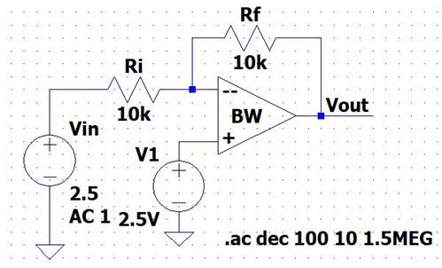
LTSpice:
Output:
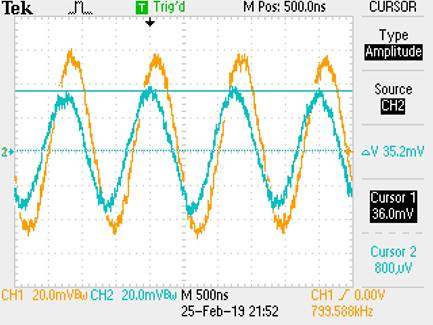
Bandwidth = 800kHz
LTSpice Output:
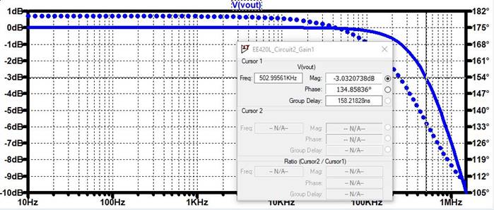
Bandwidth =
502kHz
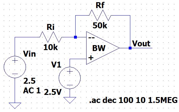
Gain of -5:
We replaced
the Rf with 50k and kept Ri = 10k
LTSpice:
Output:
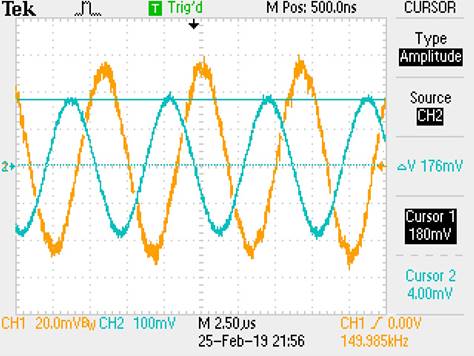
Bandwidth = 150kHz
LTSpice Output:
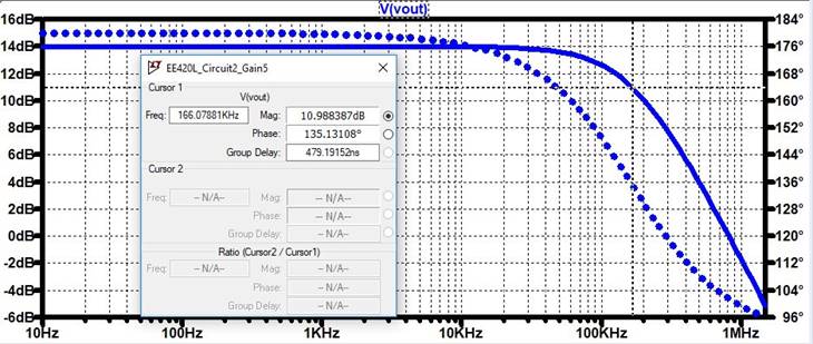
Bandwidth = 166kHz
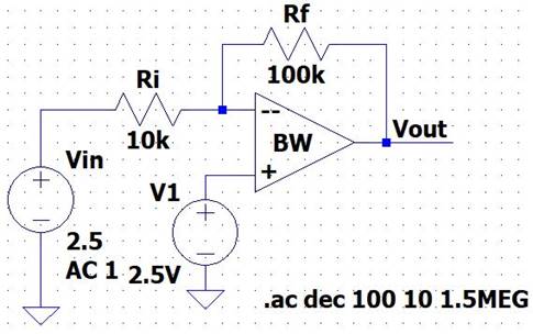
Gain of -10:
We replaced Rf
with 100k and kept Ri = 1k
LTSpice:
Output:
Bandwidth = 83kHz
LTSpice Output:
Bandwidth =
90kHz
|
Gain |
-1 V/V |
-5 V/V |
-10 V/V |
|
Experimental |
800kHz |
150kHz |
83kHz |
|
Hand Calc |
650kHz |
217kHz |
118kHz |
|
LTSpice (Ideal) |
502kHz |
166kHz |
90kHz |
Fromm the
table, we are a bit off when we are dealing with lower gains, but as the gains increase,
our Experimental and hand calcs get closer to each other. On the other hand, we
can see that the ideal LTSpice simulation is also
getting close to our experimental results as we increase the gain.
------------------------------------------------------------------------------------------------------------------
Experiment 3: The Slew Rate
In this
experiment, we will be building 2 simple circuits, a unity follower circuit
with a square input, and a unity follower circuit with a sine input. For that
we will do the following circuit:
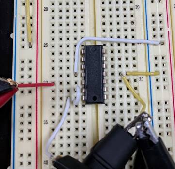
NOTE: This is the non-inverting topology
with an AC input at 2.5V DC offset.
We will be
sending a Square wave through the Op-Amp so that we can visually see the slew
rate of the Op-Amp.
For that, we
decided to stop increasing the frequency until we start seeing a “triangle”
wave.
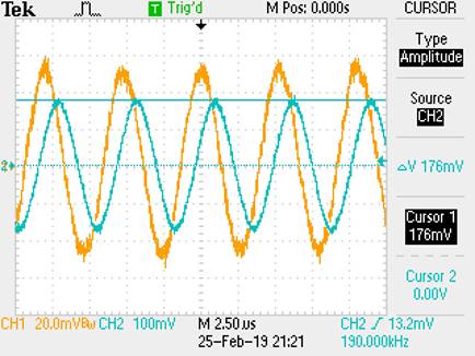
Output:
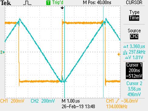
From the cursors
that we placed onto the blue output, we can use our old formula friend:
Slew Rate = Rise (Voltage difference) / Run (Time difference)
From the cursors
(and measured difference using the Oscilloscope):
1.01V
Voltage difference / 3.36us Time difference
= 301 mV/us = .3 V/us
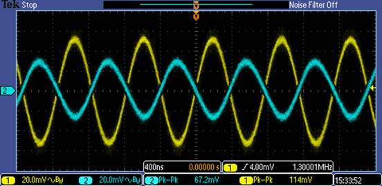
In the next
circuit, we will be changing the input from a square wave into a sine wave:
For the sine
wave, we can mathematically hand calculate this. Taking a derivative of the
sine wave, we will be left with:
2πf*Vin ≤
Slew Rate
So, given an
input of 1V, and from the datasheet, we have a Slew Rate of .4 V/us
Knowing this,
we can solve for frequency:
F ≤ SR
/ (2πVin) = (.4/10^-6) / (2π) =
63.6 kHz
Output:
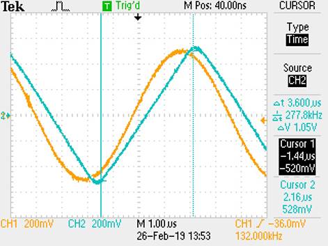
From cursors:
1.05V Change / 3.6us Change = 292
mV/us = .292 V/us
From looking at
both the slew rates of the Square wave and the sine wave, we can conclude that
the slew rate for this Op-Amp is 300 mV/us = .3 V/us
|
Input |
Slew Rate |
|
Square Wave |
.301 V/us |
|
Sine wave |
.292 V/us |
|
Datasheet |
.4 V/us |
From the table,
we can conclude that our experimental slew rate is close enough to our
datasheet slew rate.
Since this is a
parameter that is built-in to the Op-amp, the parameter is experimental
throughout many other Op-amps, just like from Lab 3, where our Voffset voltage was different between different Op-amps.