Final Project - ECE 421L
Project (not a group effort, each student will turn in their own project) – design, layout, and simulate a digital receiver circuit that accepts a
high-speed digital input signal D and Di (a differential pair connected to your circuit from, for example, a twisted pair of wires such as in an
Ethernet cable). D and Di are complements so, for example, if D is 5V then Di is 0V and output = 1. Another example, when D is 1V and Di is 2V
then output = 0. At high-speeds and long distances the voltages received aren't full digital logic levels (i.e., 5V and 0V), hence the need to design,
and use, a high-speed digital recevier circuit. Ideally, when D > Di the receiver outputs a 1. When D < Di the receiver outputs a 0. Base your
design on the topology seen in Fig. 18.23. Try to design for high-speed and low-power. Characterize your design (in sims) and the trade-offs.
For example, show that you get higher-speed if you use more energy (burn more power). See if you can get, in this 500 nm process, 250 Mbits/s
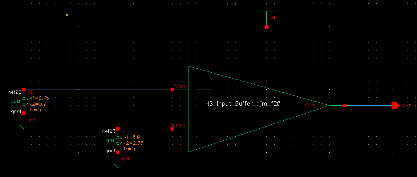
(a bit width of 4 ns) with an input voltage difference of, for example, 250 mV (with D and Di swinging back and forth between 2.75V and 3V,
for one of many examples, your circuit outputs the correspondingly correct values). Note that while Fig. 18.23 shows one inverter on the output
you may find, for example, that two inverters work better (at the cost of power). Use a table to summarize your design's performance.
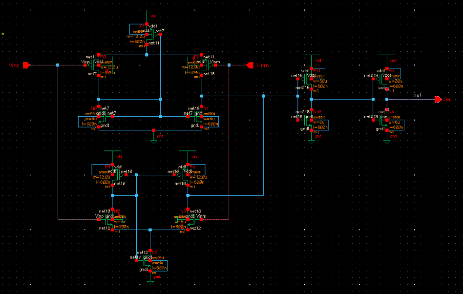
| Schematic |
|
| Symbol |
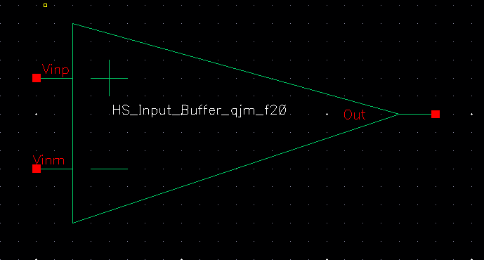 |
| Layout |
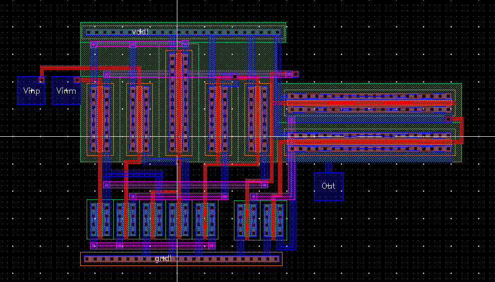 |
| LVS |
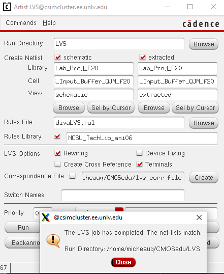 |
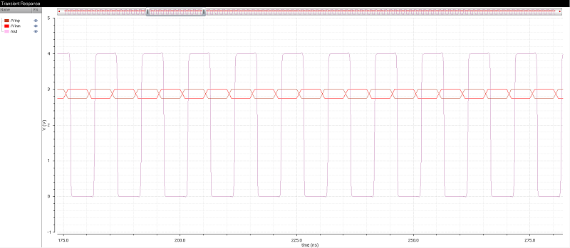
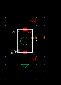
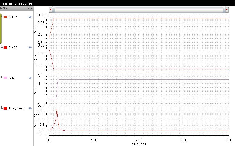
| Simulation |
 |
4ns pulse width; 1ns rise and fall time; 10ns period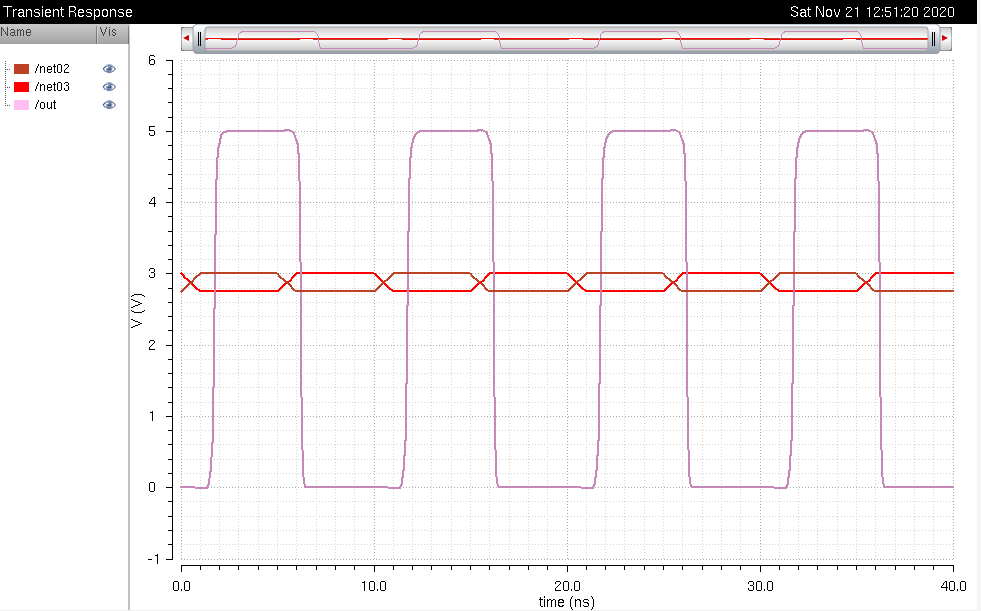 |
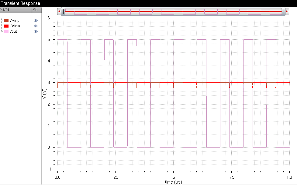
Different Input Frequency: 40ns pulse width; 100ns period
 |
 |
 |
| Power Analysis |
Plotted Power Output of the Schematic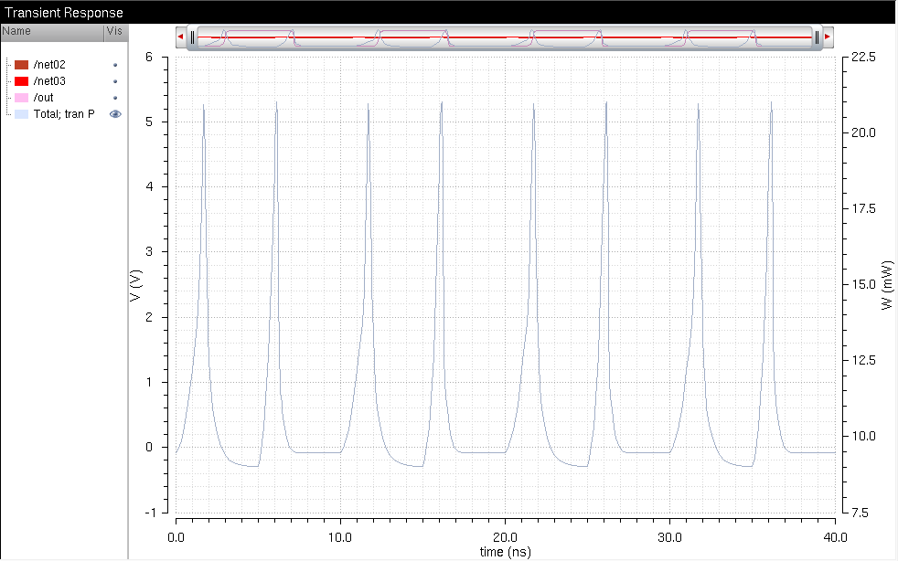 |
Average Power Calculated using Calculator 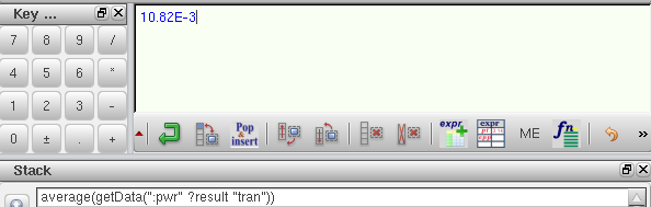 |
Here, we will show that power consumption is a function of current and therefore also temperature.
Power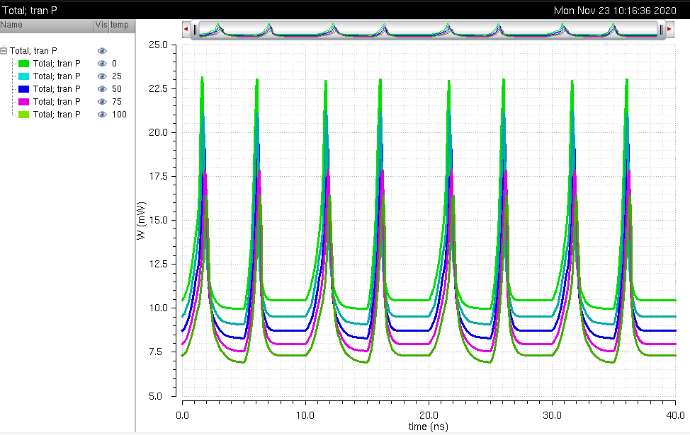 |
Labeled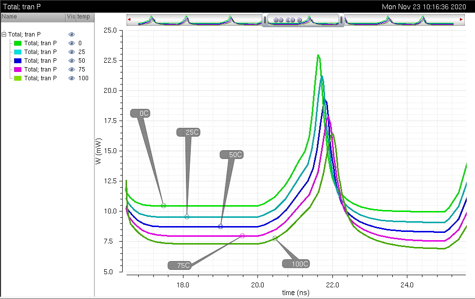 |
Here we can clearly see the relationship between the two.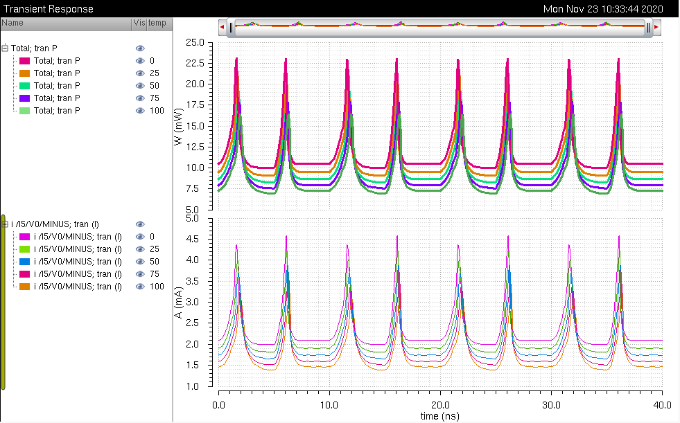 Zoomed in view showing the correlation 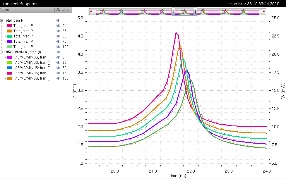 The following data shows the average power values decrease as temperature increases. 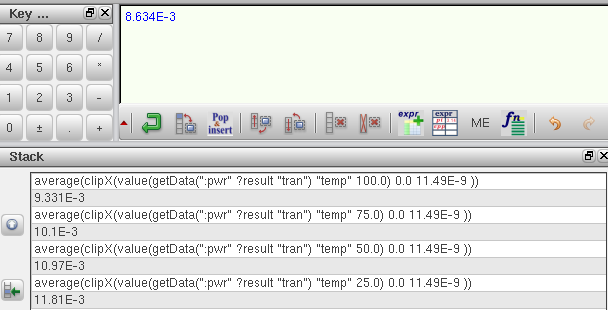 Analysis used 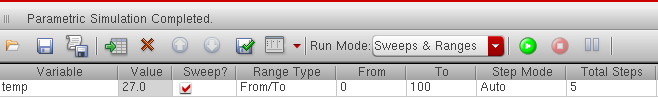 |
| Pulse Width = 100ns; Period = 200n; Measured over the same 40ns as above. |
 Here we can see that drastically slower speeds drastically cut power consumption within the same time period |
Increasing the period of measurement to 1us instead of 40ns results in a nearly the same average power consumption as above: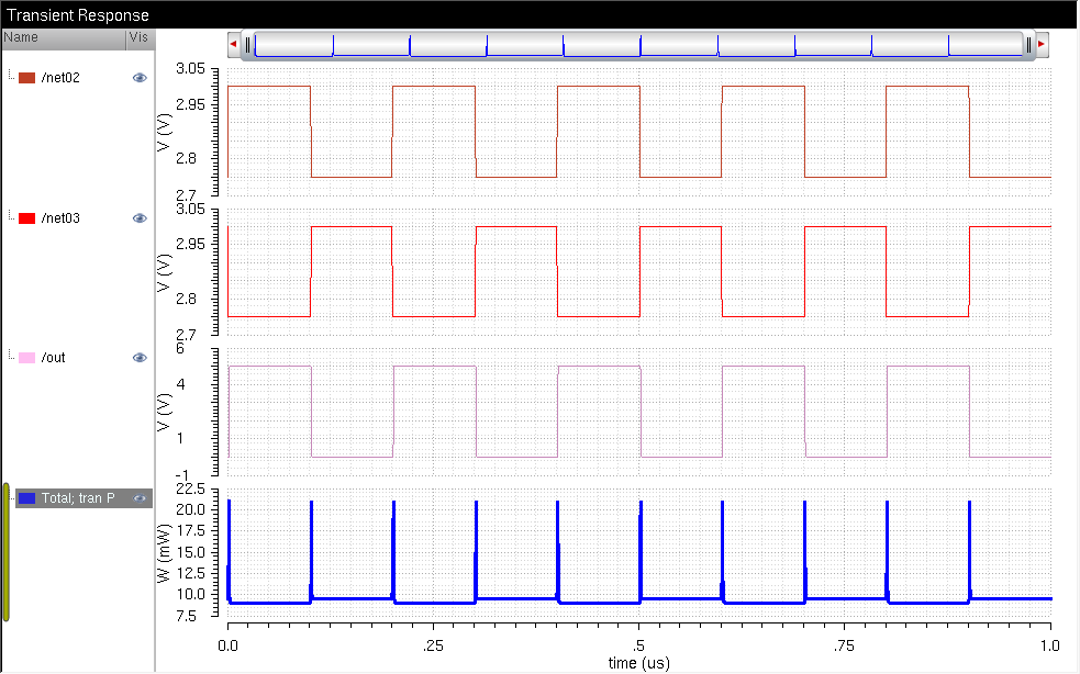 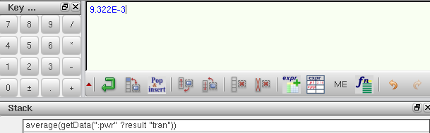 |