Lab 4 - ECE 420L
Authored
by Kyle Butler, butlerk2@unlv.nevada.edu
2/27/2019
Pre-lab work:
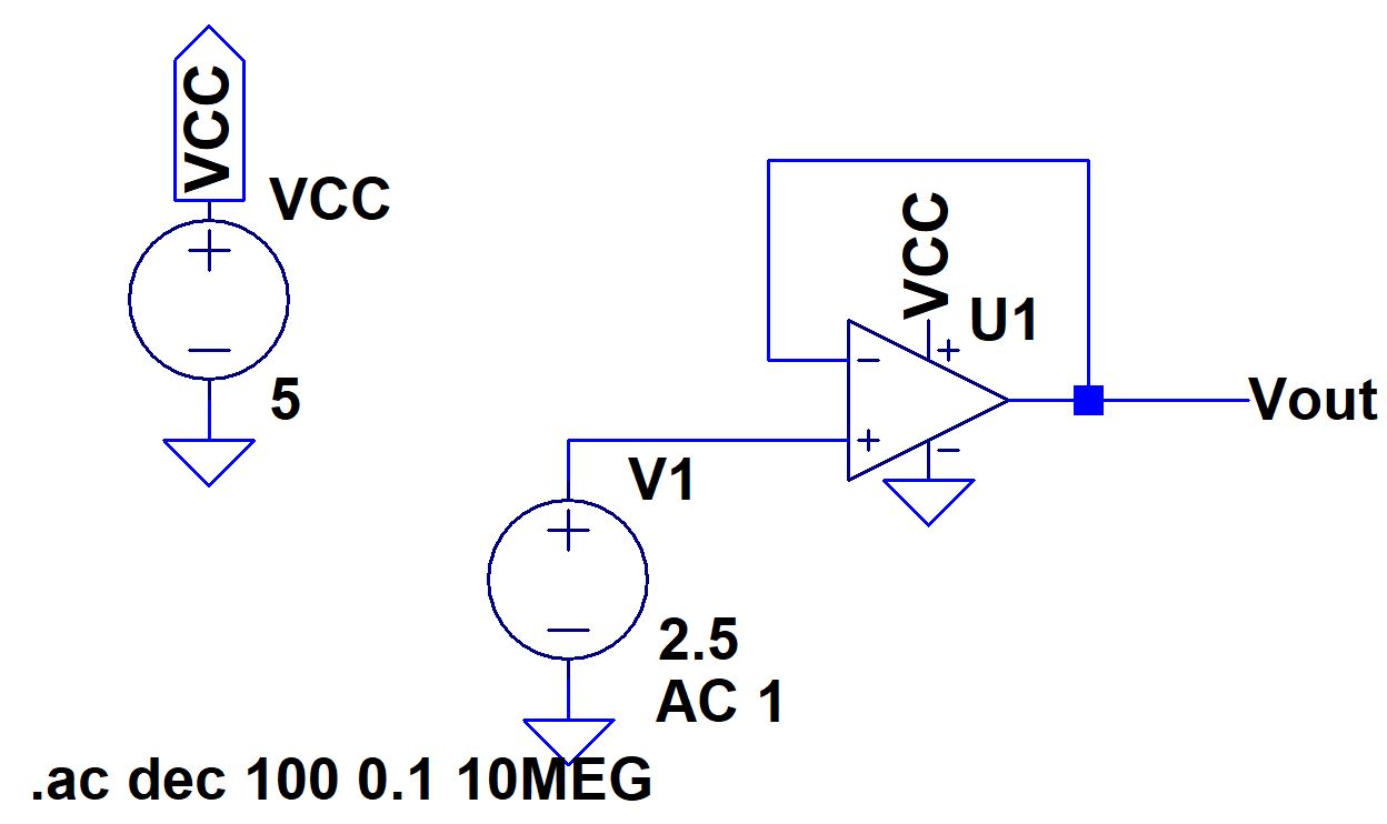
- Watch the provided video and review the associated notes. Simulate the circuits provided in the zip file.
- Read the write-up seen below before coming to lab.
Lab work:
- Estimate, using the datasheet, the bandwidths for non-inverting op-amp topologies having gains of 1,5, and 10.
- Experimentally verify these estimates assuming a common-mode voltage of 2.5V.
- Your
report should provide schematics of the topologies you are using for
experimental verification along with scope pictures/resutls.
- Associated comments should include reasons for any differeneces between your estimates and experimental results.
- Repeat these steps using the inverting op-amp topology having gains of -1,-5 and -10.
- Design
two circuits for measuring the slew-rate of the LM324. One circuit
should us a pulse input while the other should usa a sinwave input.
- Provide comments to support your design decisions.
- Comment on any differences between your measurements and the datasheet's specifications.
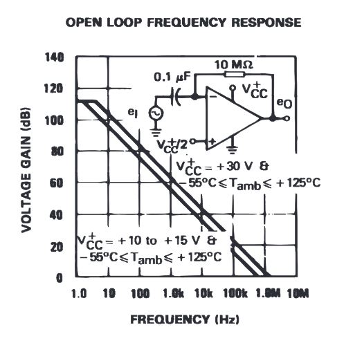
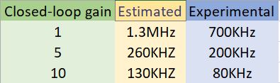
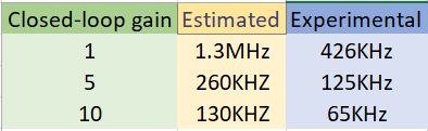
Datasheet Gain Estimation:
From
the datasheet for the LM324 the GBP of this opamp is 1.3MHz. From the
open loop frquency response wer can see at unity gain frequency is
approximately 1.3MHz

If we consider the relationship between unity grain frequency, bandwith, and gain we can find the bandwith for a given gain.
fun = Gain * Bandwith Bandwith = Gain/fun
Gain of 1:
1.3MHz = 1.3MHz/1
Gain of 5:
260KHz = 1.3MHz/5
Gain of 10:
130KHz = 1.3MHz/10
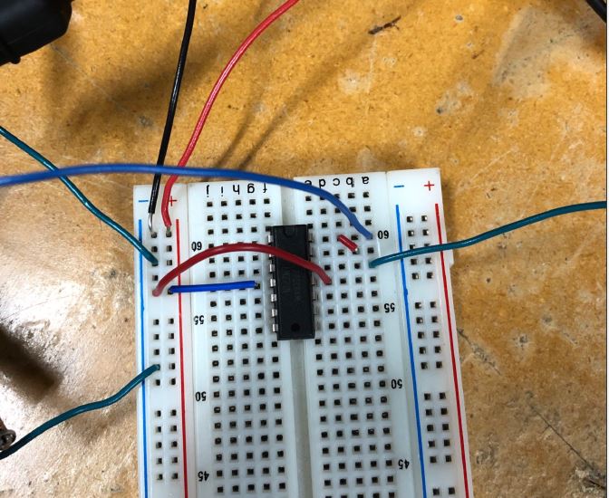
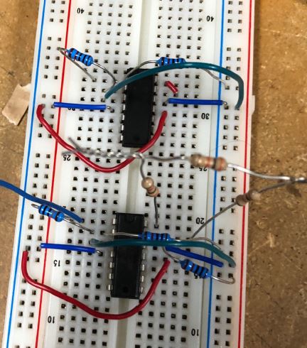
Experimental Gain Measurement
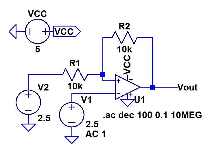
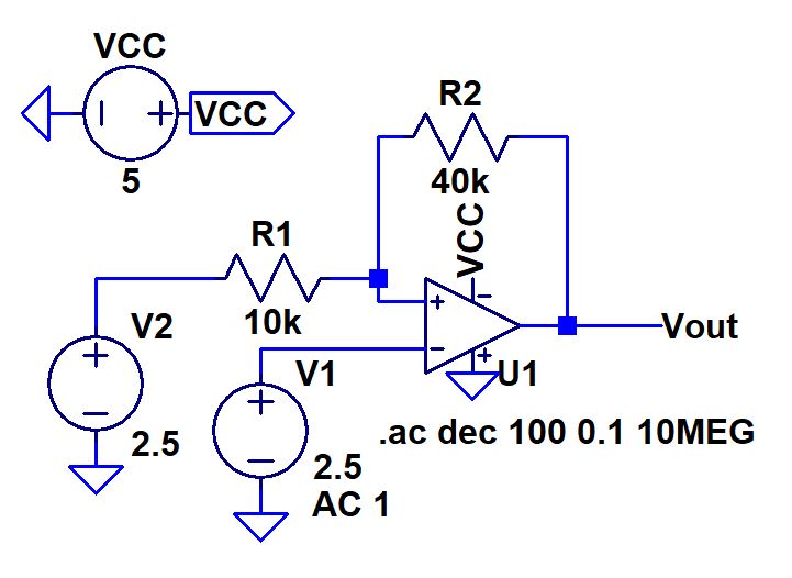
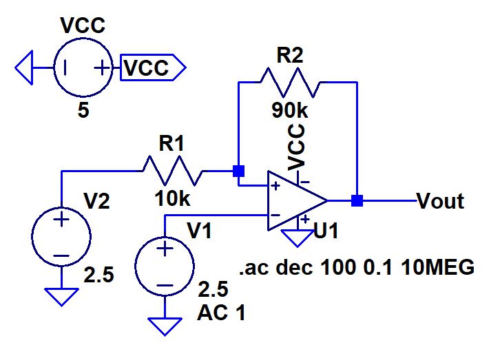
Schematics used: Gain of 1, 5, and 10 respectively
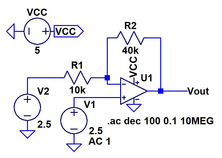
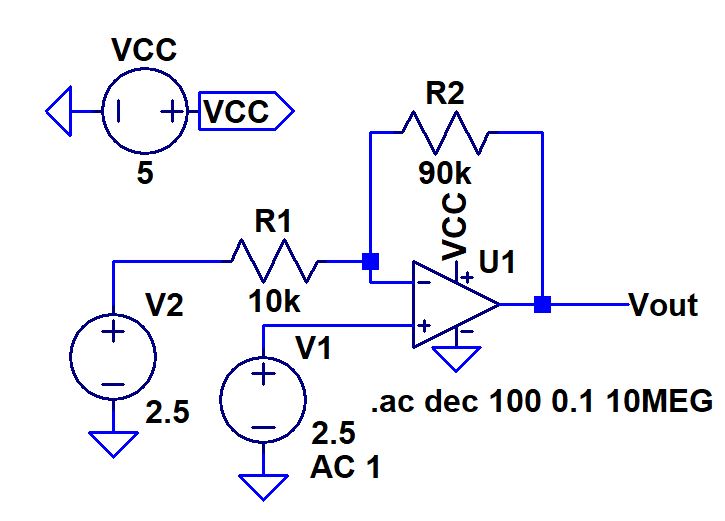
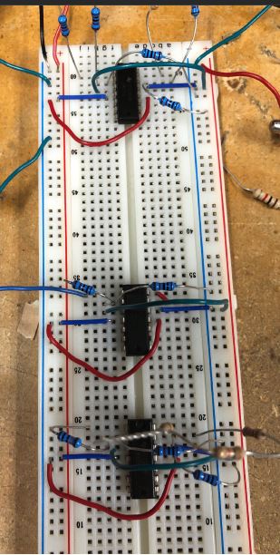
Real
world circuit: Gain of 1 and 5, for a gain of 10 the 40k was replaced
with 100k and in my haste I forgot to take the picture.
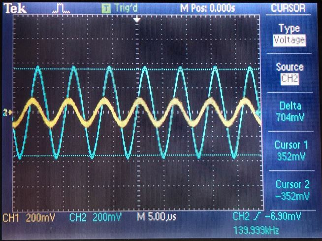
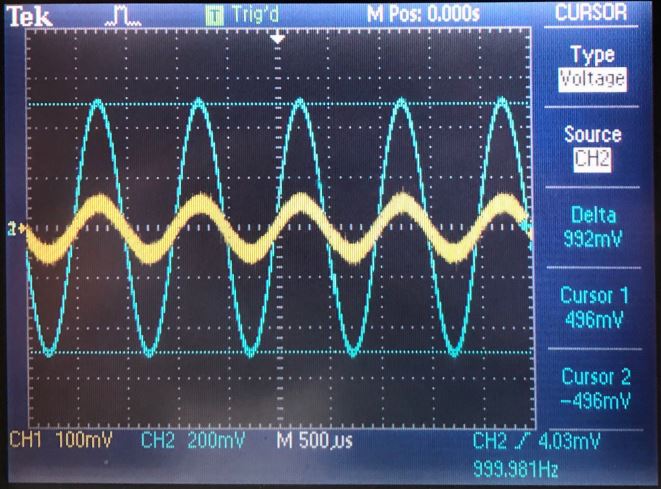
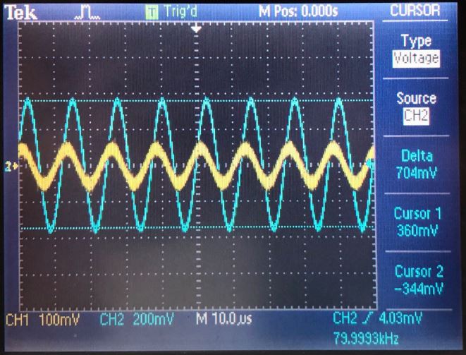
Scope pictures:
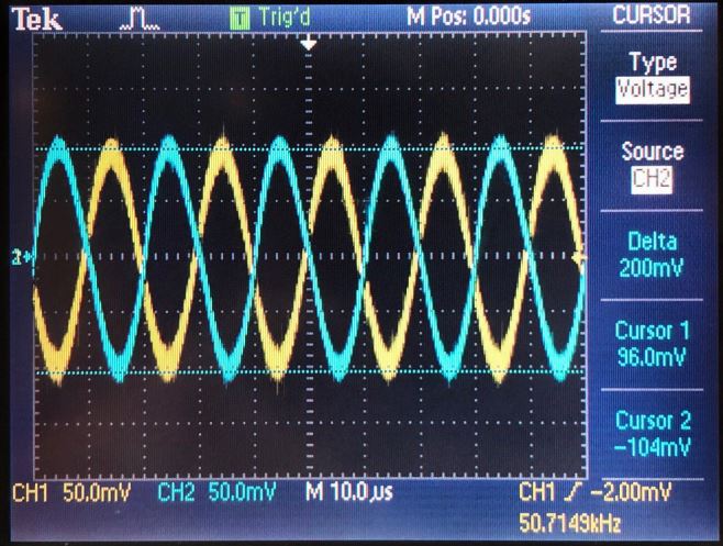
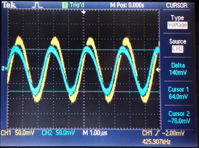
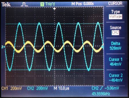
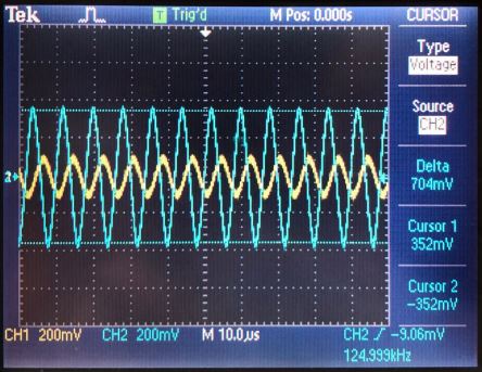
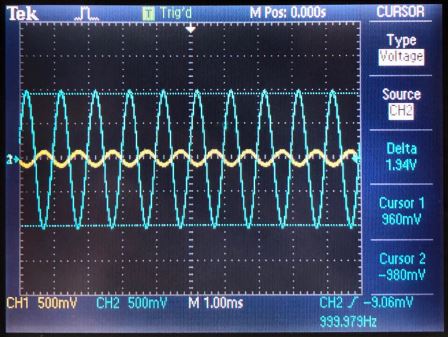
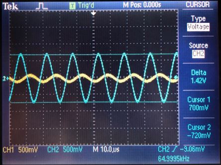
In
order to find the bandwith we chose to increase frequency until the
output is 0.707 or -3dB the input. this is the gain bandwith
Gain of 1:

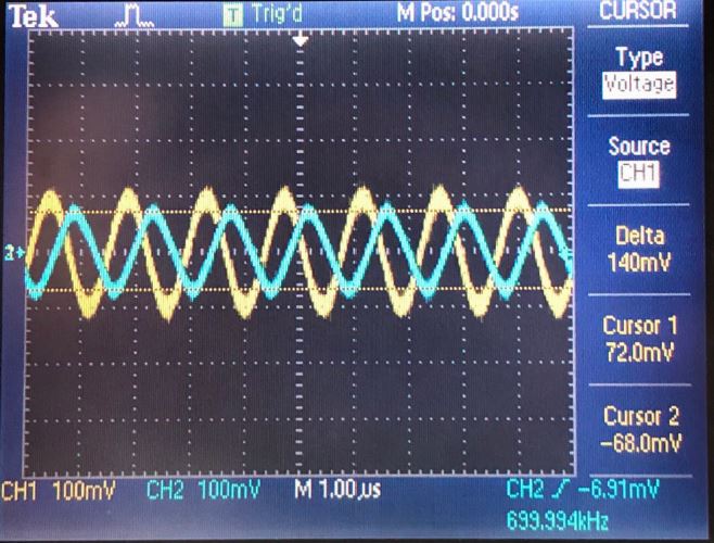
Gain of 5:
Gain of 10:
Estimated vs. Experimental bandwiths:
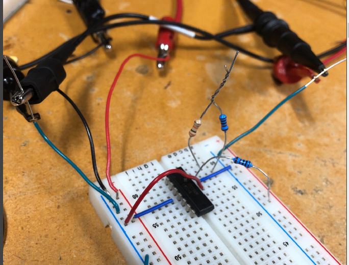
Experimental Gain Measurement(inverting)
Schematics used: Gain of -1, -5, and -10 respectively
Real world circuit: Gain of 1, 5, and 10 respectively
Scope pictures:
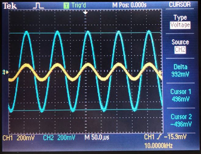
Similarly to the non inverting gains we chose to increase frequency until the
output is 0.707 or -3dB the input. this is the gain bandwith
Gain of -1:
Gain of -5:
Gain of -10:
Estimated vs Experimental bandwiths:
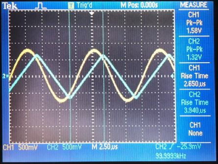
Skew Rate
First lets consider the slew rate so we can know what value of slew rate we should expect to measure

In order to measure the slew rate we will look at change in output voltage with respect to time.
Circuits builts to measure slewrate:
Scope: Square wave and Sinwave respectively
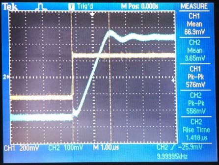
Square slew rate = 500mV/1.4uS = 0.35V/uS which is close to the 0.4V/uS slew rate
Sin slew rate = 1.5V/3.9US = 0.38V/uS which is even closer to the 0.4V/uS slew rate
Return to EE 420L Labs