Lab 4 - ECE 420L
Authored
by Stephanie Silic
silics@unlv.nevada.edu
February 22nd, 2017
Lab Description
This lab is a discussion of the bandwidth and slew rate of op-amps, using the LM324 op-amp.
This report includes the following sections:
- Part 1: Gain-Bandwidth product, Non-inverting and inverting topologies
- Part 2: Slew Rate
Lab Report
Part 1 - Gain Bandwidth Product
The bandwidth of an op-amp is the range of frequencies where it's
closed loop gain is constant. At a gain of 1, for example,
say in an inverting topology, we say its bandwidth is the
frequency where its gain starts to drop. The point where the gain
has gone down by 3 dB is where this frequency is defined. The Gain
Bandwidth Product (GBP) is the closed-loop gain multiplied by the
bandwidth at that gain, and it is a constant. The GBP is equal to the
frequency of the op-amp at unity gain ( 1*BW = GBP), also called the unity gain frequency, fun.
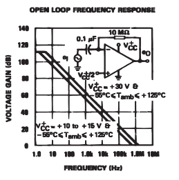
The
open loop frequency response of the LM342 is given in its datasheet. We
note that the GBP, or unity gain frequency should be around 1 MHz:
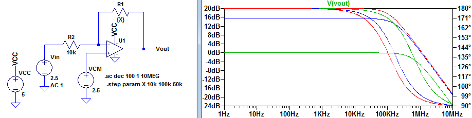
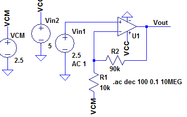
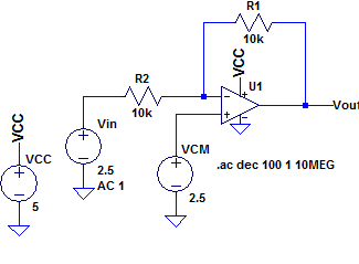
The
following circuit and simulation illustrates the frequency response of
an inverting topology at gains of 1, 5, and 10.
We note from the frequency response shown above that the bandwidth gets smaller as gain increases.
- Estimate, using the datasheet, the bandwidths for non-inverting op-amp topologies having gains of 1, 5, and 10.
The Gain Bandwidth Product (GBP) of the LM324 op-amp is 1.3MHz at Vcc=1.3MHz. This
means that its bandwidth at a certain gain can be calculated as
1.3MHz/gain. The bandwidths at gains of 1, 5, and 10 can be estimated
as follows:
- Gain of 1: bandwidth = 1.3MHz,
- Gain of 5: bandwidth = 260kHz
- Gain of 10: bandwidth = 130kHz.- Experimentally verify these estimates assuming a common mode voltage of 2.5V.
- Provide schematics of the
topologies you are using for experimental verification along with scope
pictures/results.
- Associated comments should
include reasons for any differences between your estimates and
experimental results.
Circuit used in experiment non-inverting topology, gains of 1, 5, and 10 (left to right):
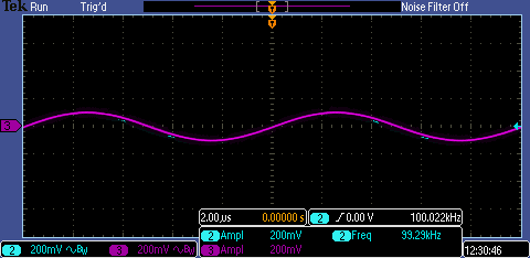
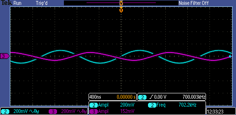
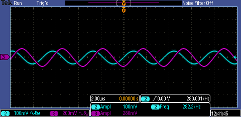
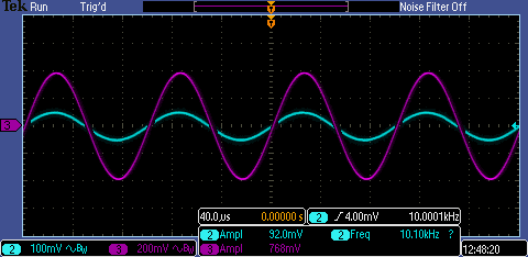
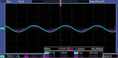
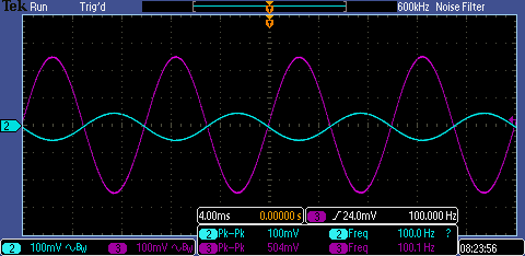
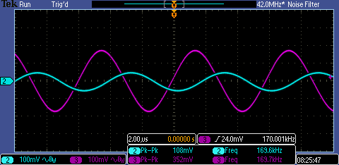
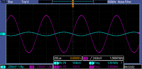
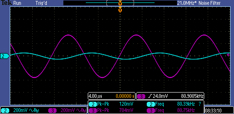
In all oscilloscope screenshots, the input is the blue waveform (channel 2) and the purple waveform (channel 3) is the output.
Gain of 1:
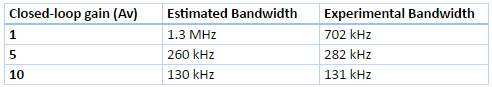
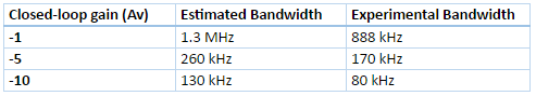
The experimental results versus the estimated bandwidths are summarized in the table below:
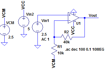
- Repeat these steps using the inverting op-amp topology having gains of -1, -5, and -10.
Inverting topology circuit used:
Again,
the screenshots on the left show the gain at a frequency within the
bandwidth, and the screenshots on the right show the gain decreased by
3dB, or when it has dropped to 70.7% of its value.
Gain of -1:
The experimental results versus the estimated bandwidths are summarized in the table below:
Part 2 - Slew Rate:
The output of an op amp can only change at a certain rate. This
rate of change is called the slew rate. On the datasheet of the LM324,
we find that the slew rate is about 0.4 V/us.
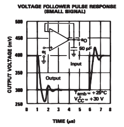
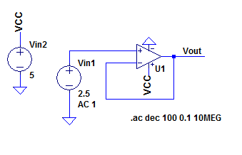
To
experimentally determine the slew rate of an op amp, we put the op amp
in the voltage follower configuration as shown in the datasheet:
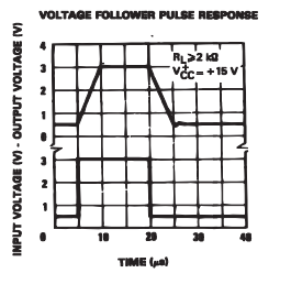
If we apply a square wave to the input of the voltage follower, the
output will not be able to change as fast as the edge of the square
wave so we will see the slew rate directly as the output changes as
fast as it can:
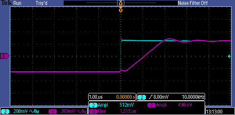
We
can calculate the slew rate experimentally from the experiment shown
above by finding the slope of the output, or change in voltage divided
by change in time. This turns out to be about 500mV/1.32 us = .37V/us which is very close to the datasheet's value of .4V/us!
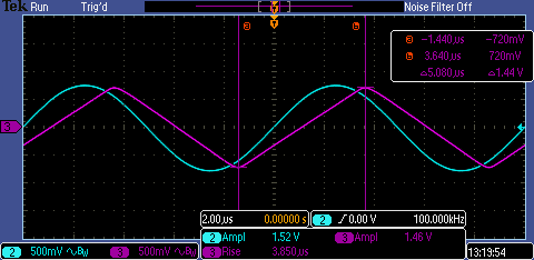
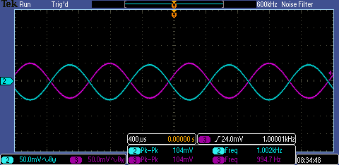
If we use a sinusoid as the input, we notice that as the amplitude of
the sine wave increases, the slope between the peaks of the sinusoid
increases as well, even at relatively low frequencies (say,
100kHz). if this slope is steeper than the slew rate, the output
of the op amp will be distorted, since it cannot change fast enough to
keep up with the sine wave. The slew rate can be seen again in the
following screenshot:
 \
\
Return to my labs


 \
\