Lab 4 - EE 420L
Desi Battle, battled@unlv.nevada.edu
2/22/2018
OP-AMPS II: G*BW and slewing
- Estimate, using the datasheet, the bandwidths for non-inverting op-amp topologies having gains of 1, 5, and 10.
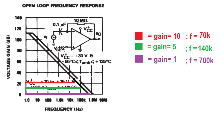
Using this chart found on pg 6/13 of the LM324 datasheet pdf I estimated the
bandwidth by noting the intersection of the given gain and the bandwidth.
Since the Gain Bandwidth product is a constant, once we find the
X-intercept, or the bandwidth for a gain of 1 (0 dB), we can use that value
to estimate the other two bandwidths since the gain is known.
Why DB?
While the equation (dB) = 20log(Vo/Vin) generates a value for gain in decibals, it doesn't really explain why.
We use dB for frequency response plots because the value of the gain exponentially falls off with increased frequency.
To make the visualization easier to represent/understand we use logarithmic axes making the actual plot linear.| Gain | Bandwidth | Bandwidth (estimated) | Gain * Bandwidth | Gain * Bandwidth (est) |
| 1 | ? | 700KHz | ? | 700 K |
| 5 | ? | 120 KHz | ? | 700 K |
| 10 | ? | 70 KHz | ? | 700 K |
| -1 | ? | 700 KHz | ? | 700 K |
| -5 | ? | 140 KHz | ? | 700 K |
| -10 | ? | 70 KHz | ? | 700 K |
EXPERIMENT 1
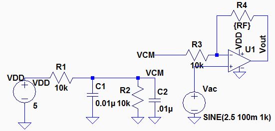
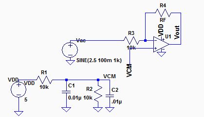
Schematic used for non-inverting bandwidth experiments.
| Experiment | RF Value (ohms) | Gain produced (Vout/Vin) |
| 1 | 0 | 1 |
| 2 | 40K | 5 |
| 3 | 90K | 10 |
Steps:
- Place components on breadboard as drafted above
- Use an oscilloscope to show the ac source and Vout at f = 1kHz and verify expected closed-loop gain
- Increase
frequency until Vout is 0.707 times its original value and record this
value as the 3db frequency (the frequency where Z{Re} = Z{Im})
Repeat steps 1-3 for the six different gains listed in the table.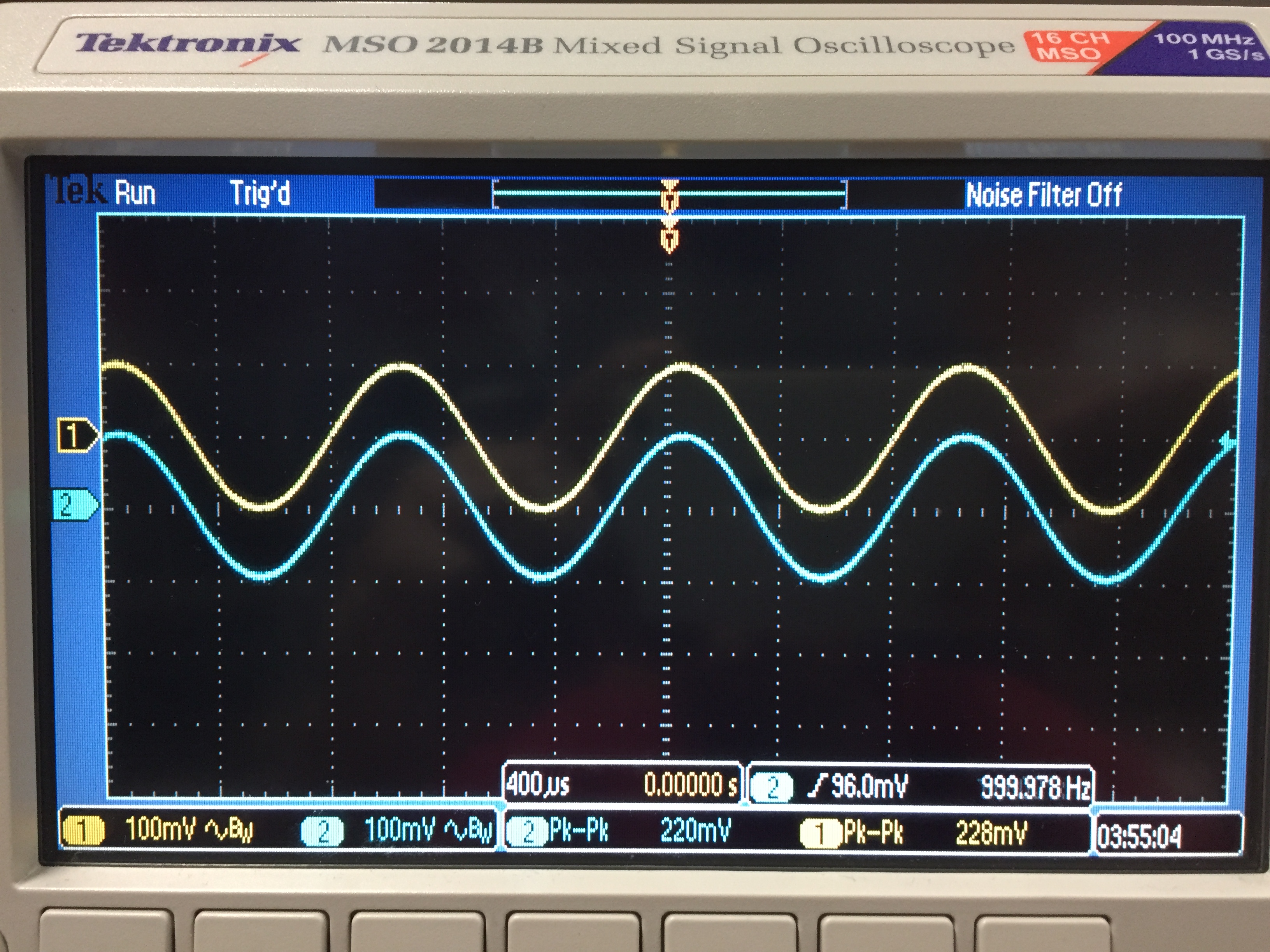
Vout
= Vin ; f = 1kHZ
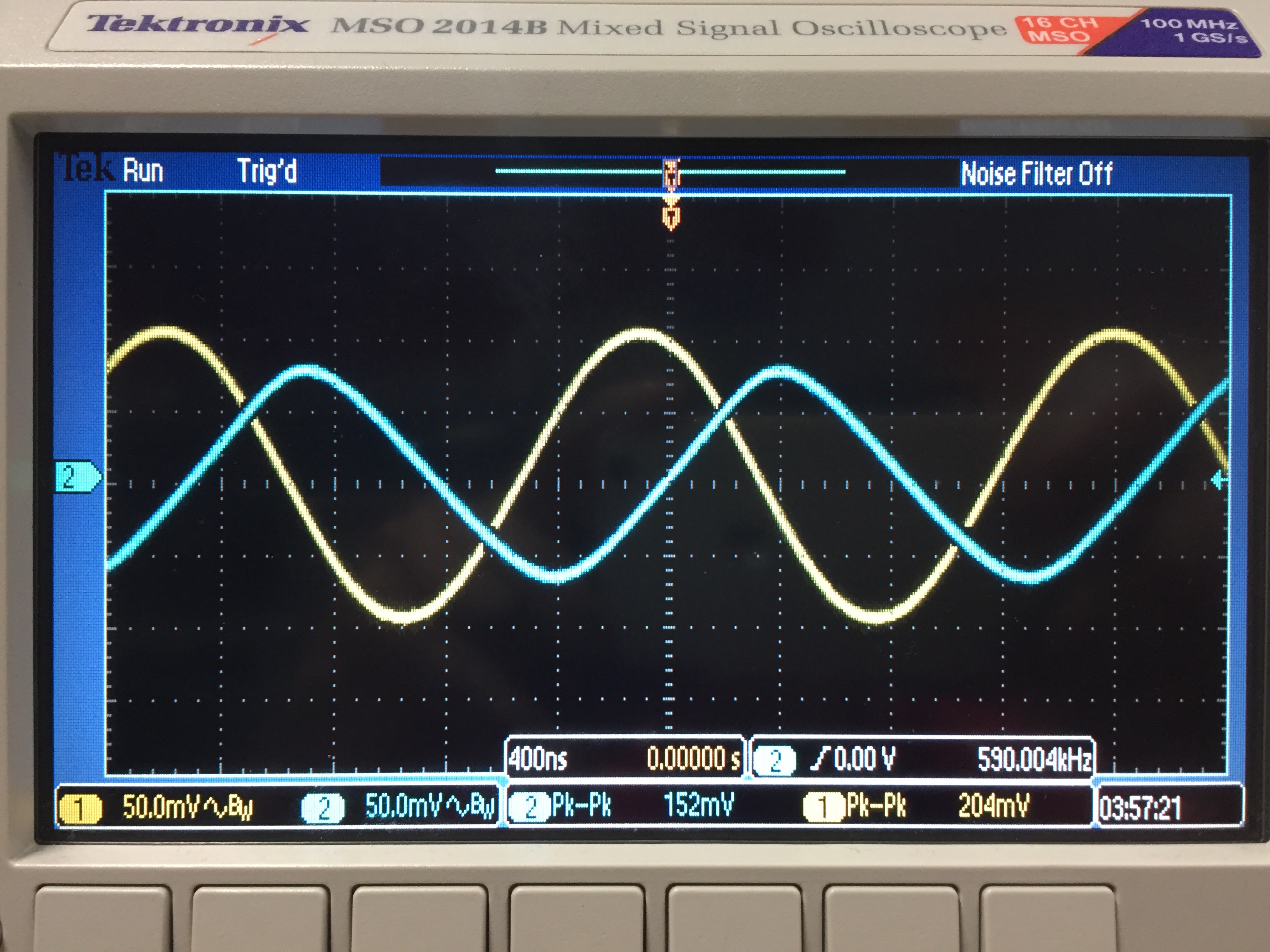
f3db = 590KHz
Start at 1KHz, increase until :
Vout = 220 * 0.707 = 156 mV or about 590 KHz
Vout
= 5*Vin ; f = 1kHZ
f3db = 177KHz
Start at 1KHz, increase until :
Vout = 900 * 0.707 = 636 mV or about 177 KHz
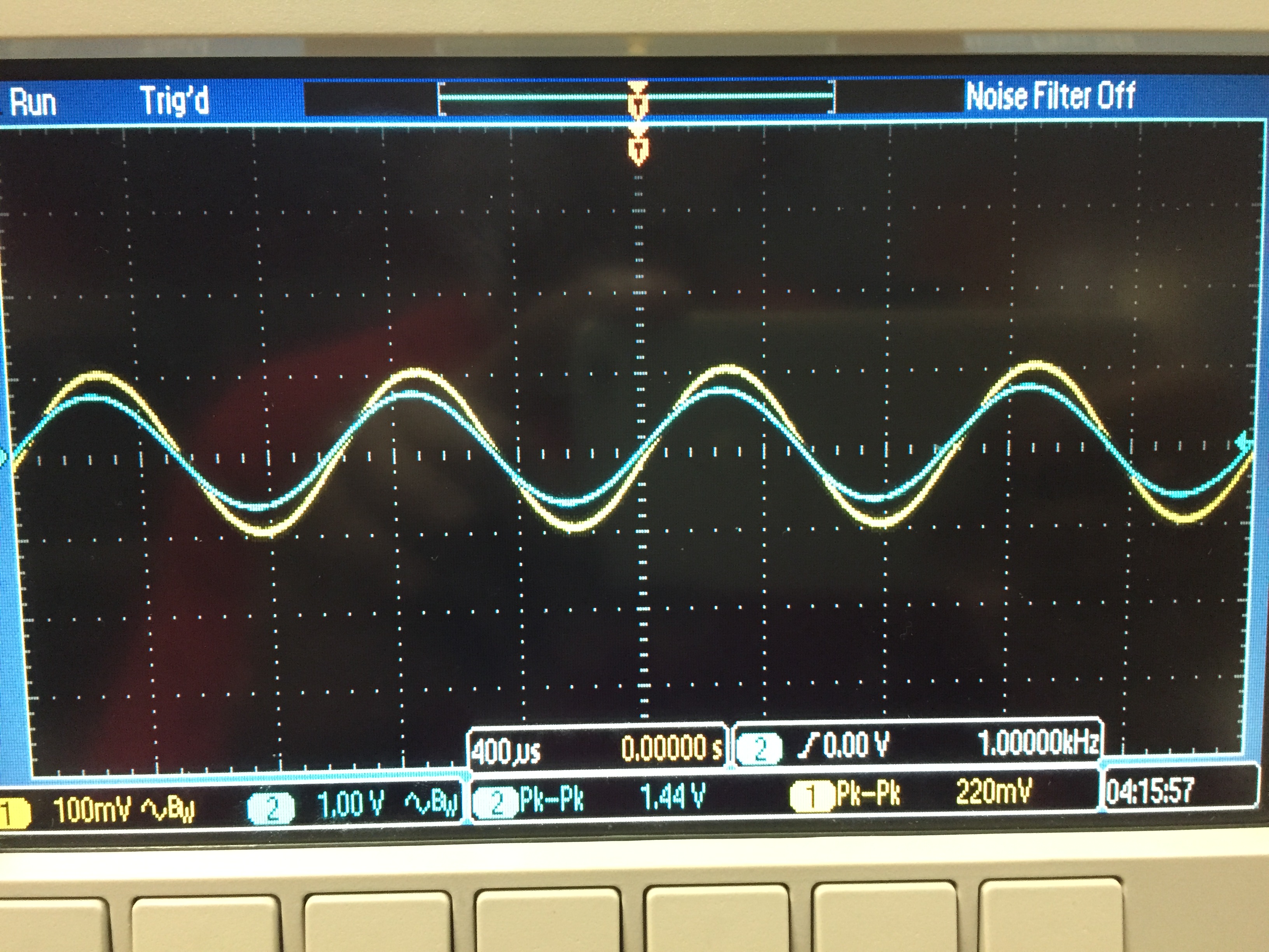
Vout
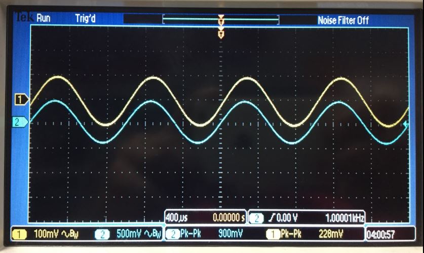
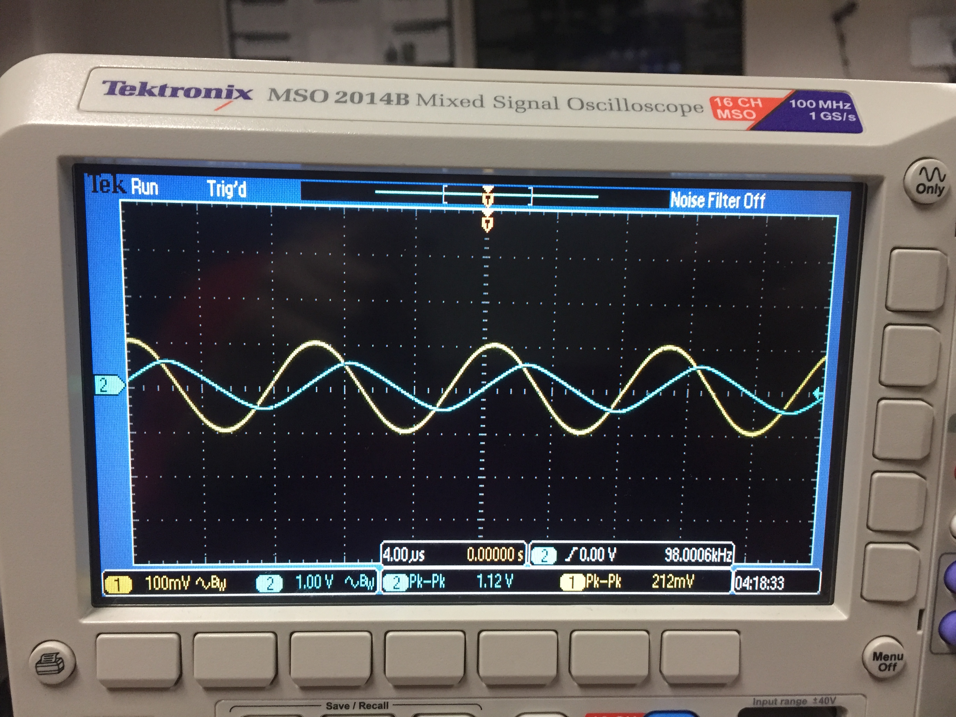
= 10*Vin ; f = 1kHZ
f3db = 98 KHz
Start at 1KHz, increase until :
Vout =1.4 * 0.707 = 1.01 V or about 98 KHz
| Gain | Bandwidth | Bandwidth (estimated) | Gain * Bandwidth | Gain * Bandwidth (est) |
| 1 | 590 KHz | 700KHz | 590 K | 700 K |
| 5 | 177 KHz | 120 KHz | 885 K | 700 K |
| 10 | 98 KHz | 70 KHz | 980 K | 700 K |
| -1 | ? | 700 KHz | ? | 700 K |
| -5 | ? | 140 KHz | ? | 700 K |
| -10 | ? | 70 KHz | ? | 700 K |
Table Summarizing results for noninverting topology
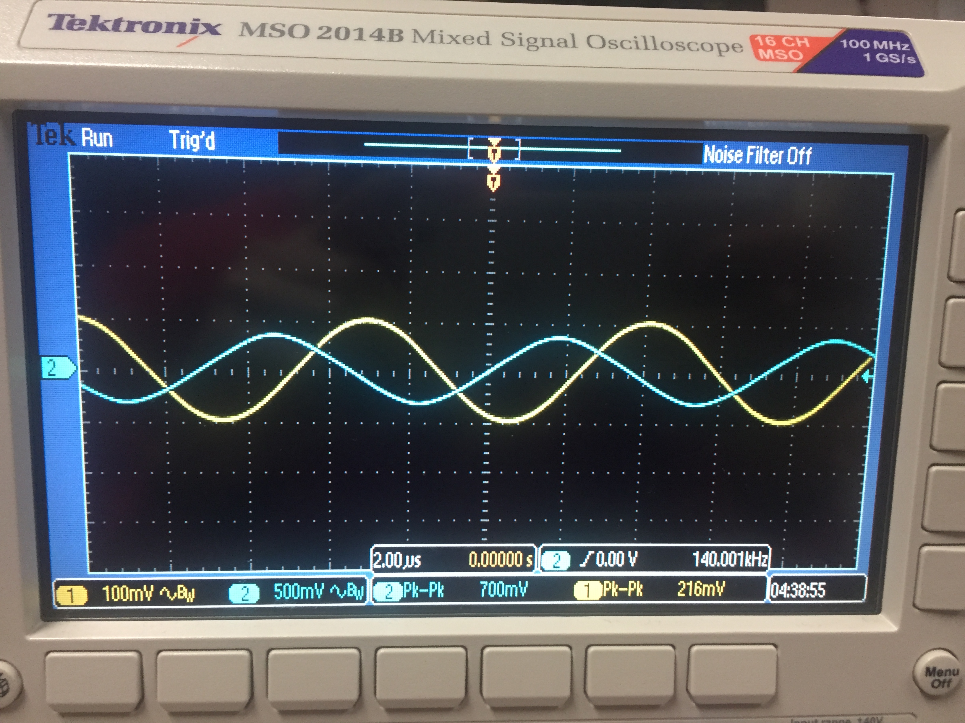
Schematic used for inverting bandwidth experiments.
| Experiment | RF Value (ohms) | Gain produced (Vout/Vin) |
| 1 | 10/k | -1 |
| 2 | 50K | -5 |
| 3 | 100K | -10 |
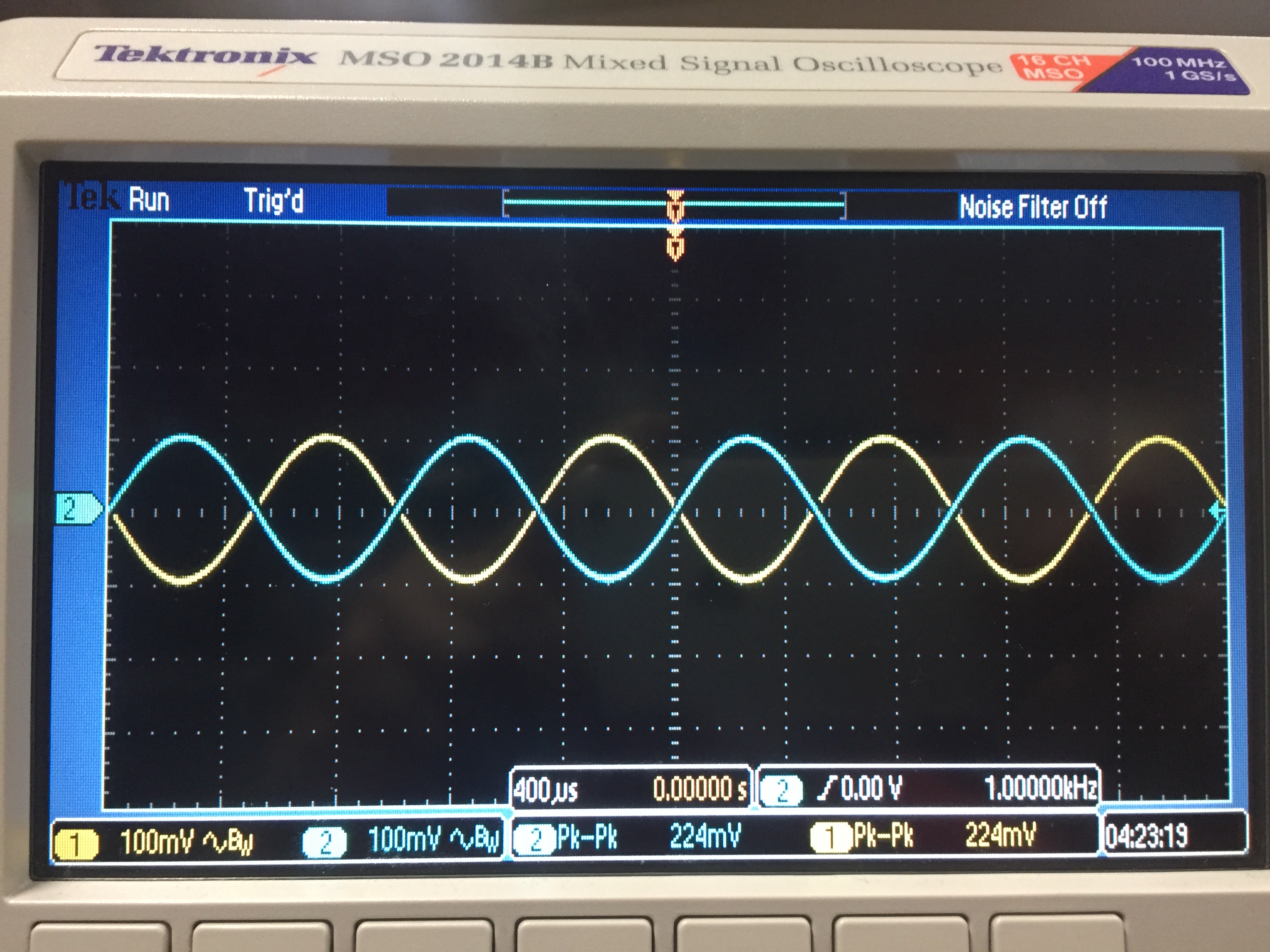
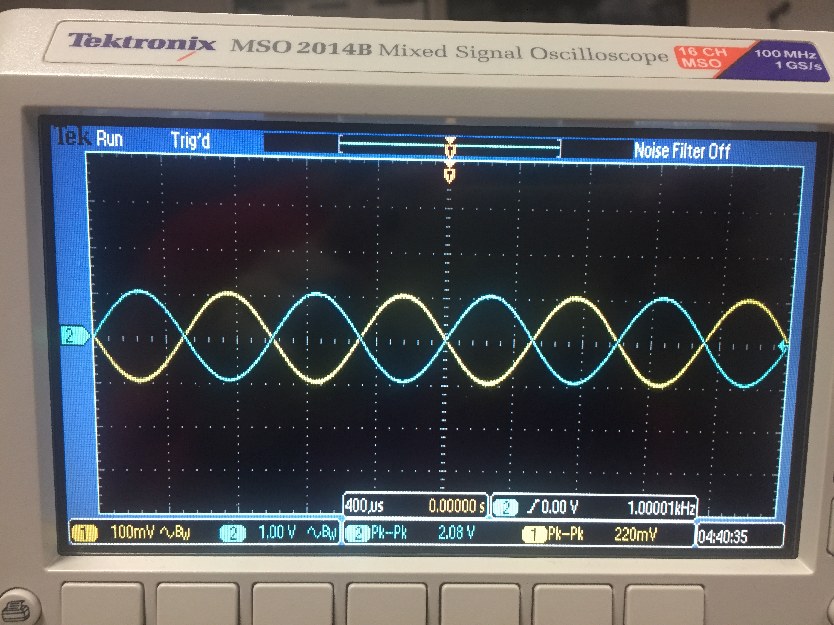
Vout
= -Vin ; f = 1kHZ
f3db = 640KHz
Start at 1KHz, increase until :
Vout =224* 0.707 = 158 mV or about 640 KHz
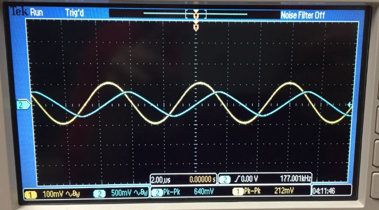
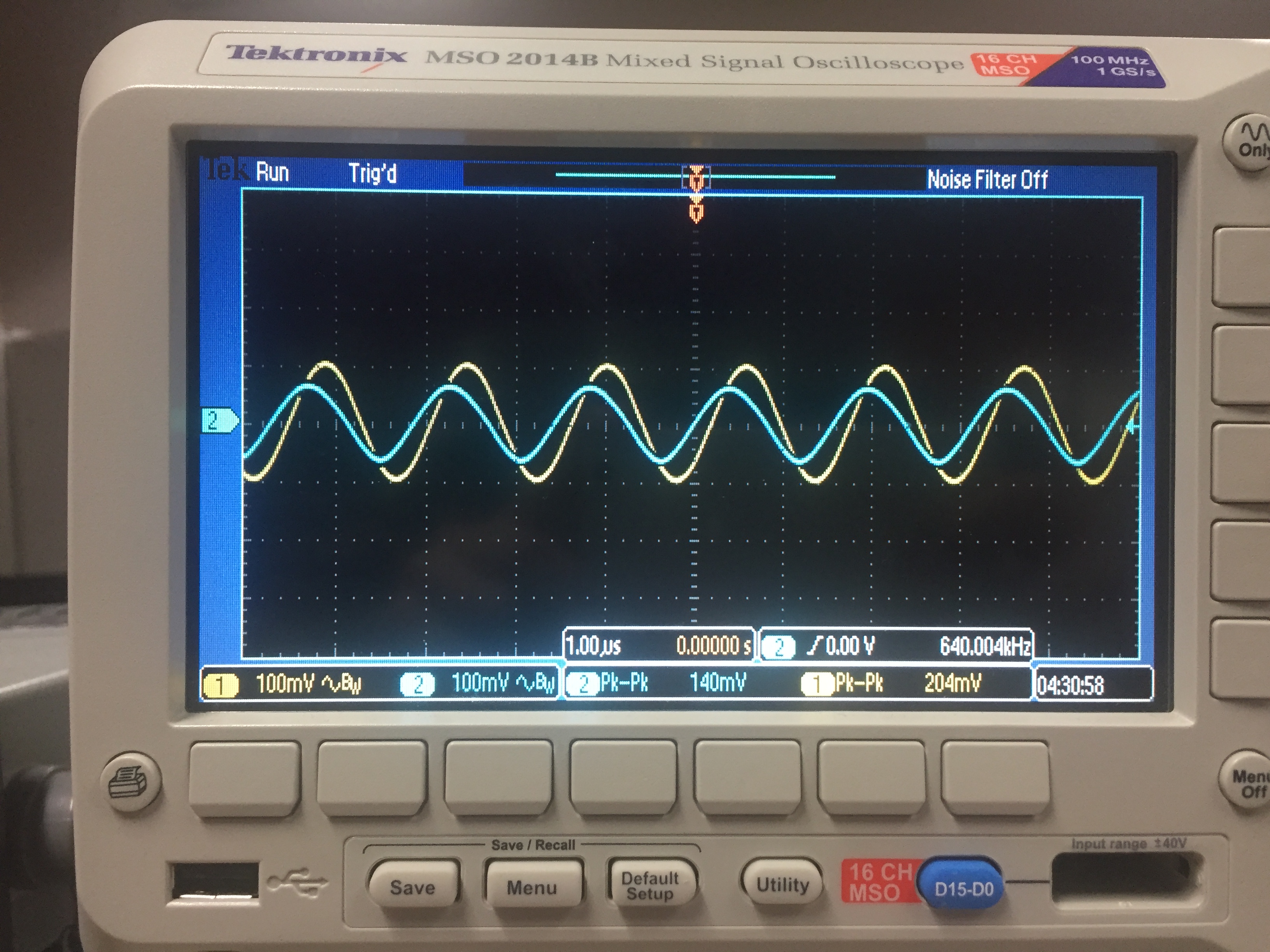
Vout
= -5*Vin ; f = 1kHZ
f3db = 140KHz
Start at 1KHz, increase until :
Vout =1.04* 0.707 = 735 mV or about 140 KHz
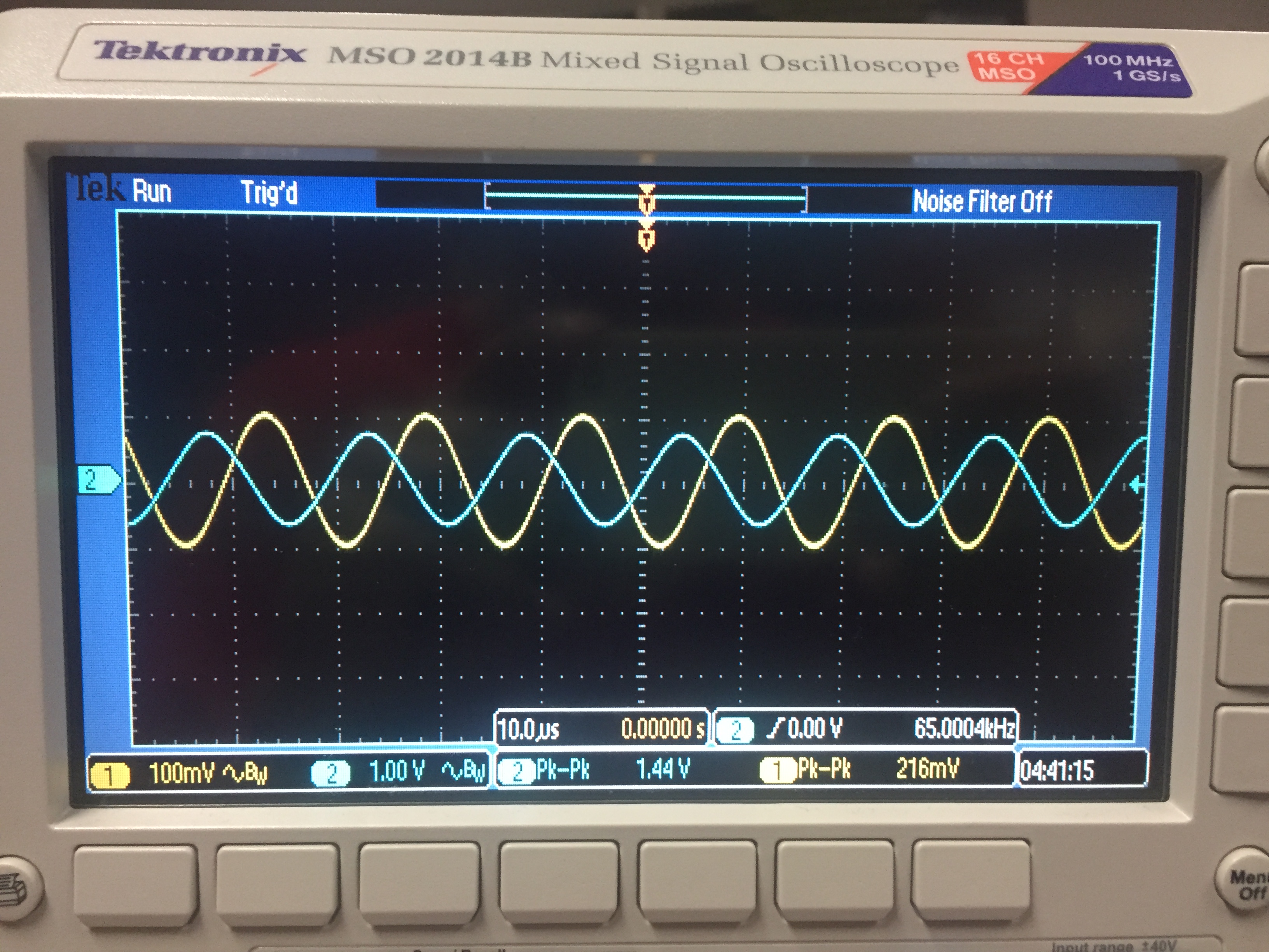
Vout
= -Vin ; f = 1kHZ
f3db = 65KHz
Start at 1KHz, increase until :
Vout =224* 0.707 = 1.47 mV or about 65 KHz
| Gain | Bandwidth | Bandwidth (estimated) | Gain * Bandwidth | Gain * Bandwidth (est) |
| 1 | 590 KHz | 700KHz | 590 K | 700 K |
| 5 | 177 KHz | 120 KHz | 885 K | 700 K |
| 10 | 98 KHz | 70 KHz | 980 K | 700 K |
| -1 | 640 KHz | 700 KHz | 640 K | 700 K |
| -5 | 140 KHz | 140 KHz | 700 K | 700 K |
| -10 | 65 KHz | 70 KHz | 650 K | 700 K |
Summary of experiment results.
Discuss:
Comparing
the inverting and noninverting topologies, we see that the
Gain*Bandwidth product of the inverting topology stayed fairly
close to
the predicted 700K, while that of the noninverting topology
ranged wildly from 590K to 980K. I believe input offset voltage and limitations of the
resolution of the oscilloscope mainly attributed to these errors.
If we take the average of all the Gain*Bandwidth products we recorded we get 740K, 40K or 6% off from our 700K estimate,
but
since the estimate just serves the purpose of a starting reference
point when choosing frequencies to probe with experimentally I find the
%error to be acceptable.
EXPERIMENT 2
To measure slew rate first we reconfigure our LM324 to be non-inverting with a gain of 1 (unity follower)
First lets use a Sine wave to get our measurement.
Start by setting the input to a 200 mV, 250KHz sine wave and ensure the output is following exactly (1)
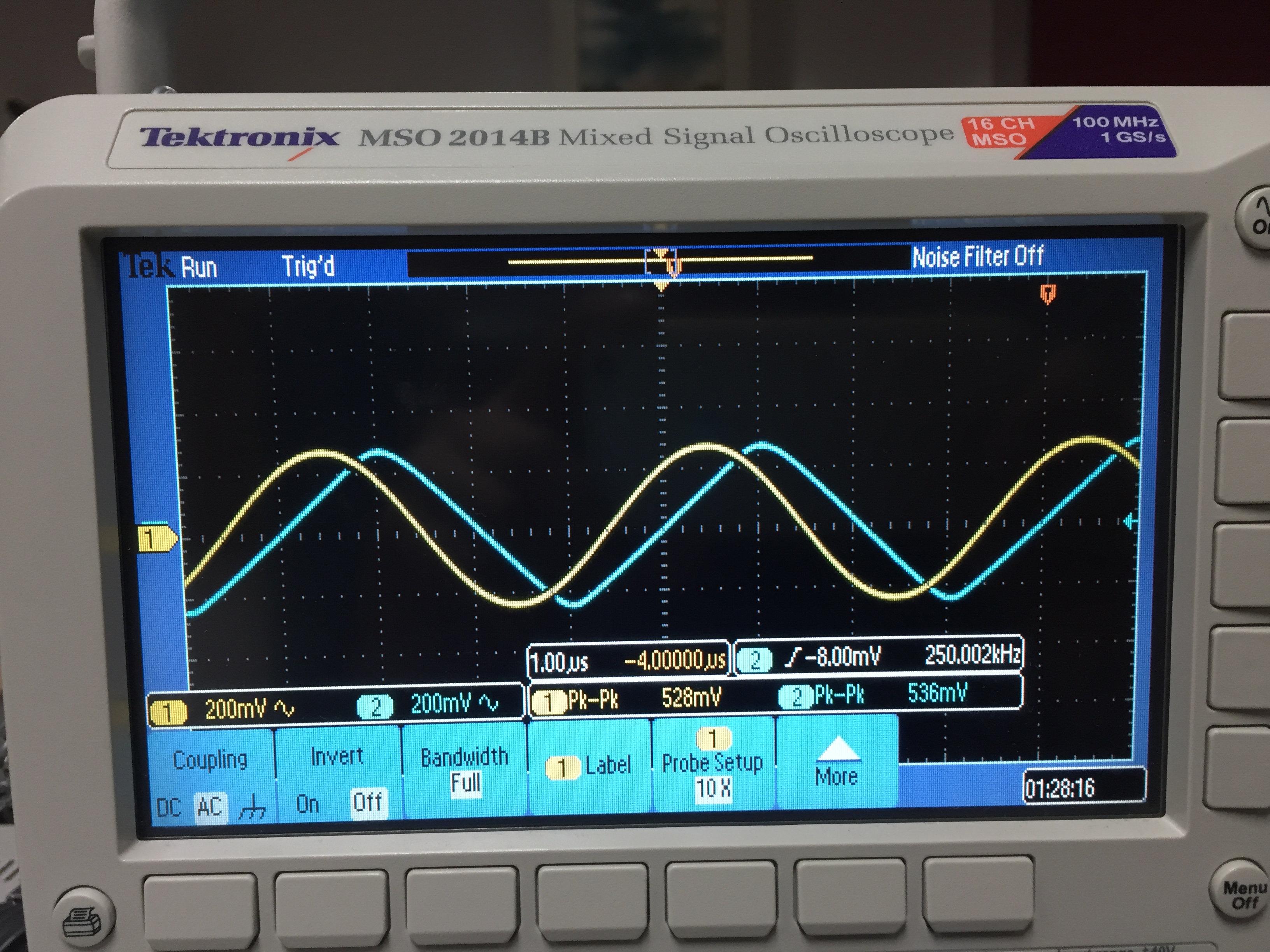
Next
slowly increase the amplitude (2a). Stop once you reach a point
where further increasing the input amplitude does not increase the
output. (2b)
Finally, using the scope cursor, measure the slope of output. This is your measured slew rate. (3)
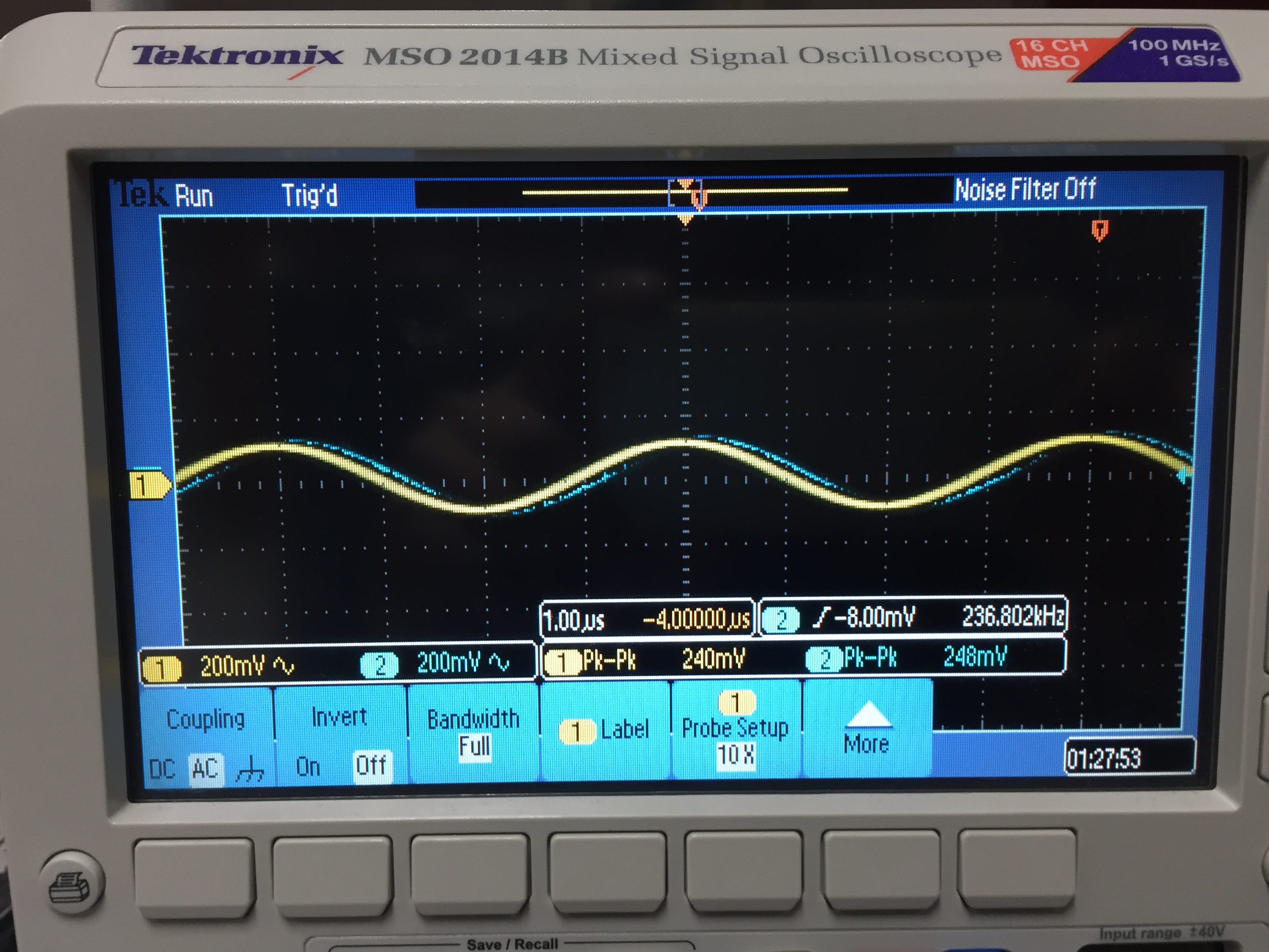
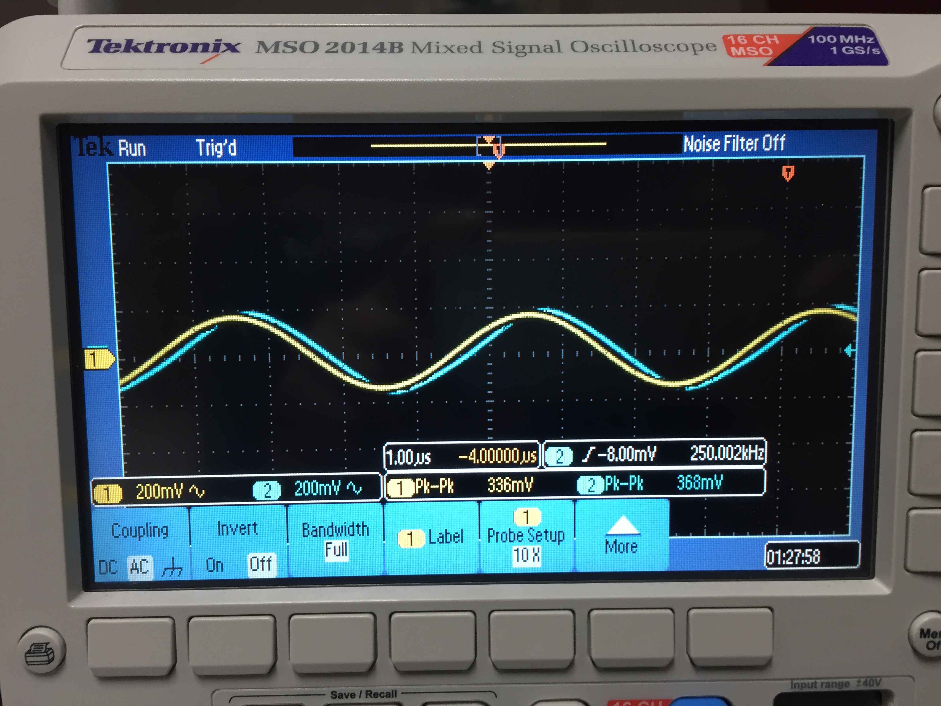
(1)
(2a)
(2b)
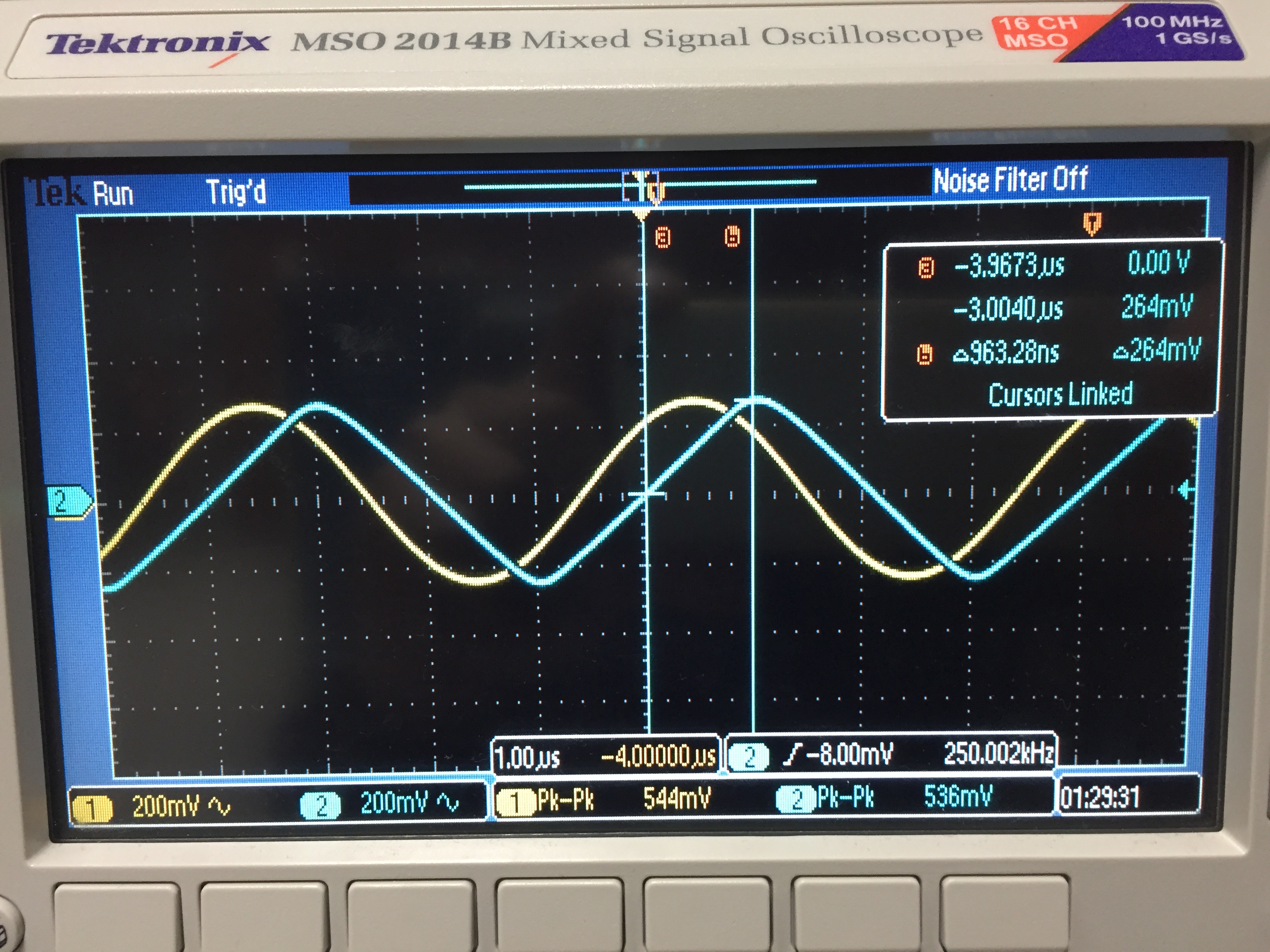
(3)
dV = 280 mV ; dt = 960 nS
Slew Rate = dV/dt = 284mV/960nS or roughly 0.3 V/us
Next, we measure the slew rate again, but this time using a pulse input instead of a sine wave.
Begin
by taking the sine source from our last measurement and change it to a
pulse, then set the pulse width to 20us and verify output is as expected (1)
increase the frequency until you can visually detect a difference between the input and output rise times. (2)
Using the measure function, calculate the rise time, then divide 0.8Vo by the rise time to measure the slew rate (3)
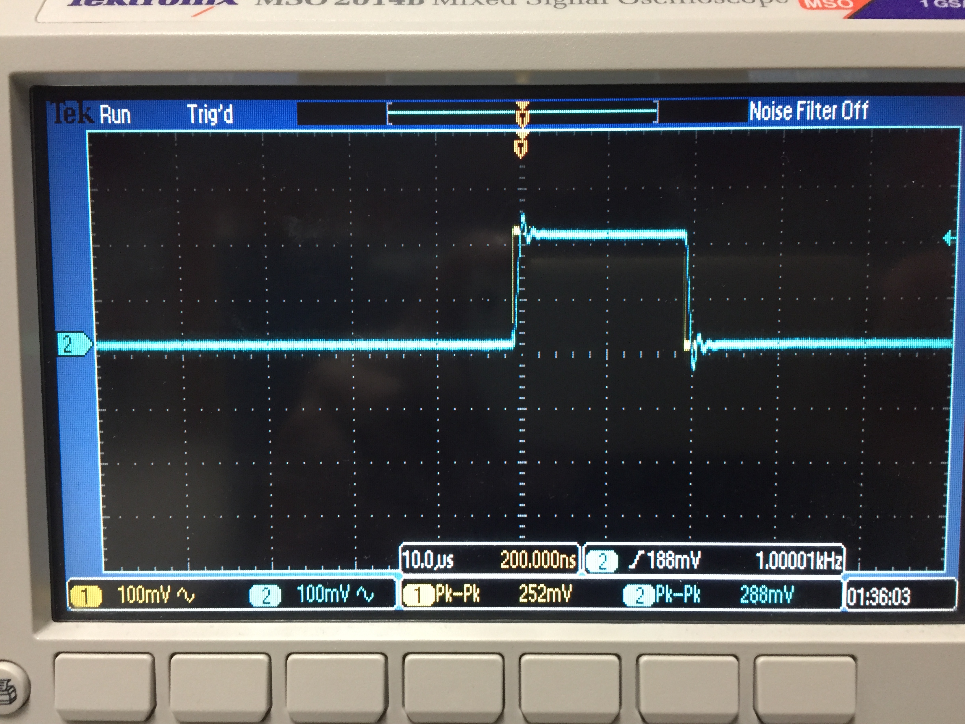
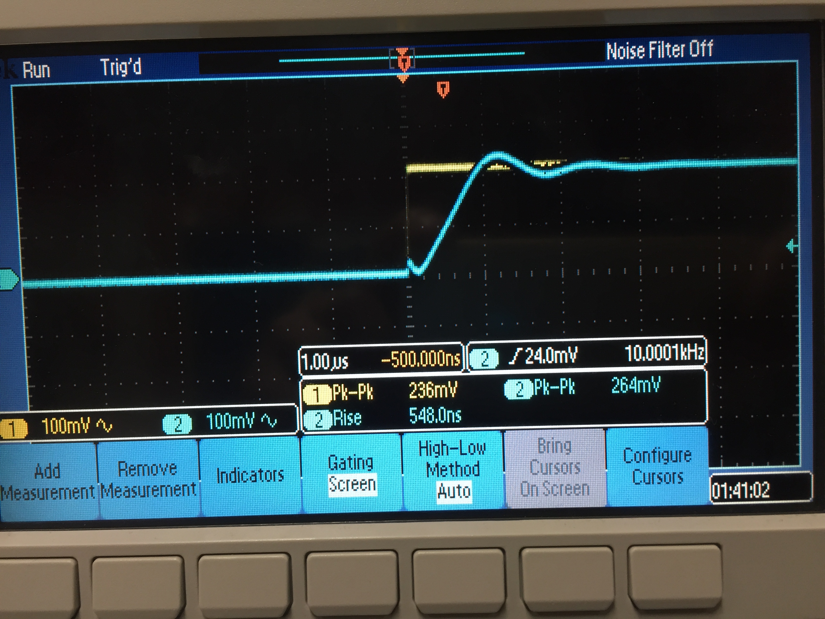
(1)
(2)
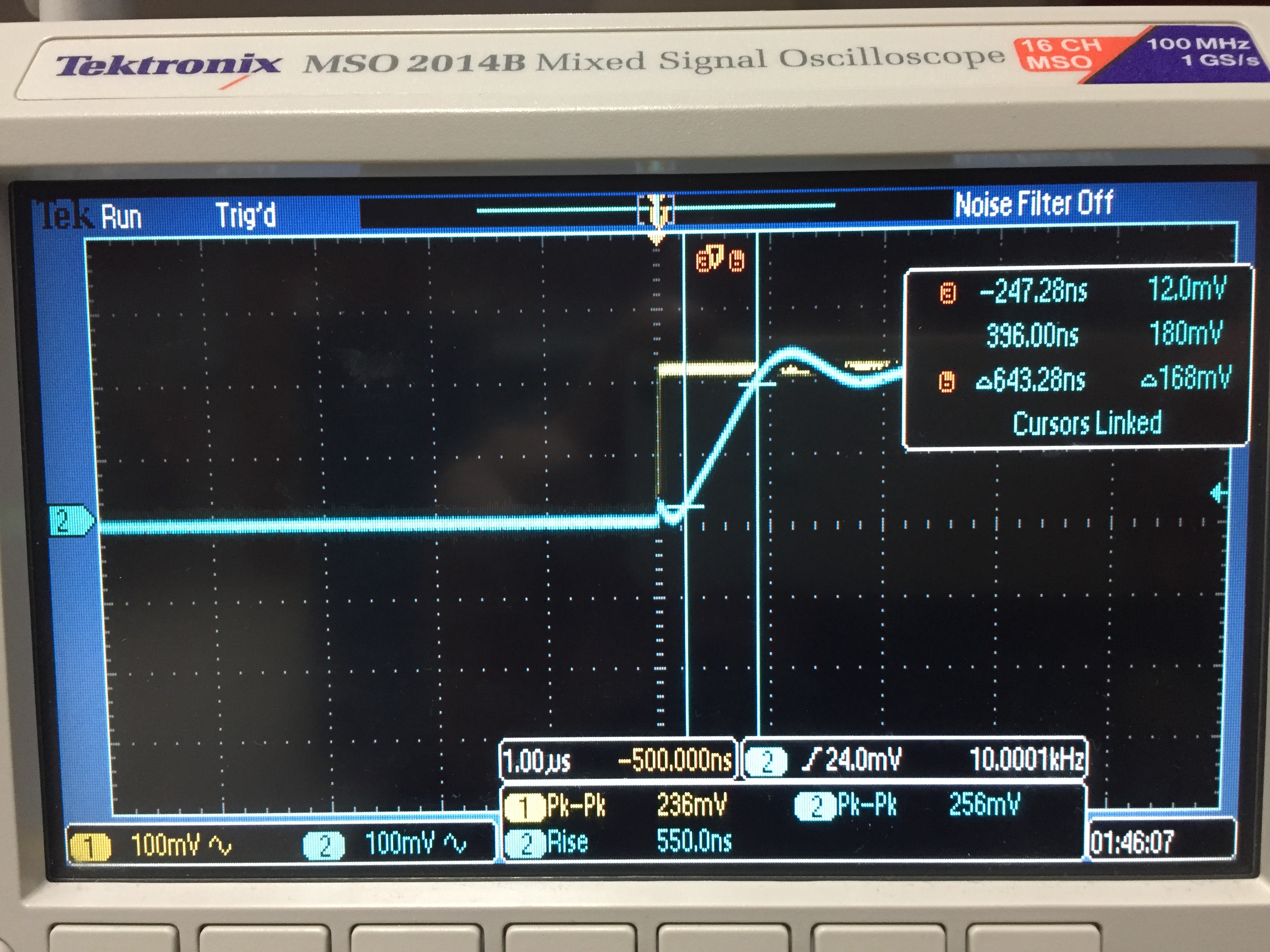
(3)
Rise = 550 ns ; Vo = 220mV
Slew Rate = Vo/Rise = 0.4V/uS
| Method | Results |
| Sine Input | 0.3 V/uS |
| Pulse Input | 0.4 V/uS |
| Data sheet | 0.4 V/uS |
Discuss:
Looking back at the experiment using the Sine input, I notice that my
error is likely introduced by erroneous measuring techniques.
The peak voltage I measure contains portions of the sine wave where the dV/dt is less than maximum rate of change, resulting in
an answer less than other methods suggest
Conclusion:
After performing this week's lab I now have the understanding that the
slew rate is essentially the limiting factor for the bandwidth of a
configuration.
It now makes qualitative sense that for a given frequency, a
given configuration will have lower bandwidth for higher gains.
If
the op-amp output can just barely produce a 100mV sine wave with a gain
of 1 at unity frequency, attempting to produce a larger signal
wont
change the output, since the output slew rate has already been reached
a larger signal cannot be generated with the given frequency.
Return to labs