Lab 4 - EE420L
Dwayne K. Thomas
kendaleman@gmail.com
2/27/2015
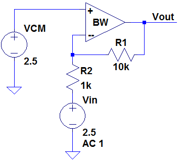
Opamps II, gain bandwidth product and slewing
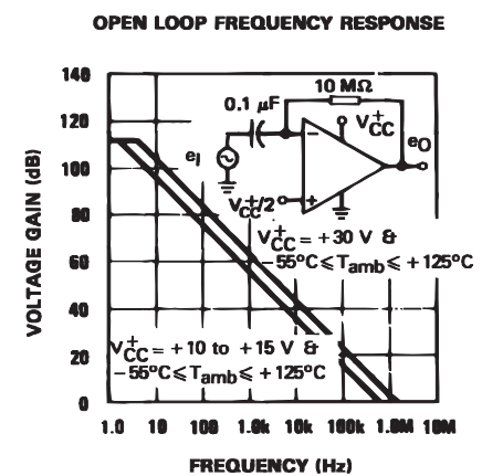
The
Gain Bandwidth
product provided by the datasheet is 1.3MHz. This means that as
our
gain is increased, the available bandwidth we have decreases linearly.
1.3MHz also marks the unity gain frequency. The plot on the
left is given by the datasheet to help us determine what our bandwidth
would be for different gain circuit htat are used with this Opamp .
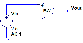
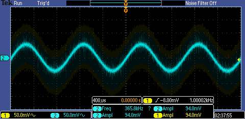
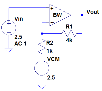
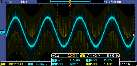
| Gain of 1 | The
estimated bandwidth of the unity gain is given by the datasheet as
1.3Mhz. The scope output on the left shows our gain of 1 at
1khz, and the scope on the right shows our reduction in output
amplitude to 66% at a little over 1MHz. |
 |  | 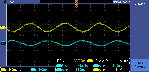 |
| Gain of 5 | The bandwidth of this topology is estimated at 260kHz. The scope output on the left shows
our gain of 5 at 1khz, and the scope on the right shows our reduction
in output amplitude to 65% at about 210kz. |
 |  | 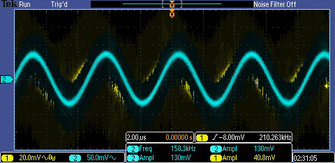 |
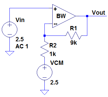
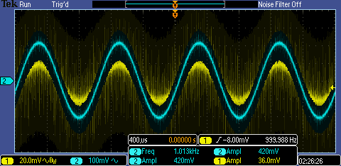
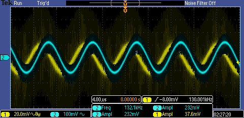
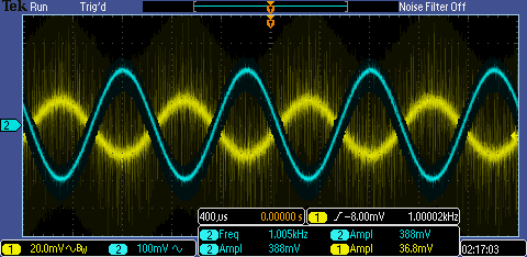
| Gain of 10 | The bandwidth of this topology is estimated as 130khz. The scope output on the left shows
our gain of 10 at 1khz, and the scope on the right shows our reduction
in output amplitude to 55% at 130kHz which indicates that our 3db frequency is much lower. |
 |  |  |
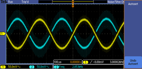
| Gain of -1 | The estimated bandwidth of this topology is 650kHz. The scope output on the left shows
our gain of -1 at 3khz, and the scope on the right shows our reduction
in output amplitude long before we reach our target frequency |
 |  | 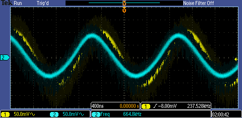 |
| Gain of -5 | The bandwidth of this topology is estimated as 216khz. The scope output on the left shows
our gain of -5 at 1khz, and the scope on the right shows our reduction
in output amplitude to 70% at about 204kz. |
 | 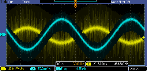 |  |
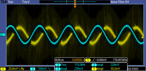
| Gain of -10 | The bandwidth of this topology is estimated as 118khz. The scope output on the left shows
our gain of -10 at 1khz, and the scope on the right shows our reduction
in output amplitude to 57% at 118kz |
 |  |  |
Our
test results indicate that the output gain bandwidth chart and
calculations are a guide to determine the what kind of bandwidth we are
limited for a specific topology and gain. We found that the
bandwidth we actually had was more limiting than our estimations in
every case. This might due to the low rail voltage of 5V used
which is much lower than what the Opamp was tested at provide the
graph. We also had inconsistencies with our function generator which
can be seen in the yellow input probe noise in each graph.
| Voltage Follower | Slew Rate limiting with Pulse input | Slew Rate limiting with sine wave |
|  |  |
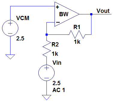
Th
reason we chose the Voltage Follower circuit to test our slew rate is
because of the simple task the Opamp has in this configuration.
Whatever voltage is placed on the input of our noninverting
terminal should be the same voltage we get on our output terminal.
In addition, there are no other circuit elements such as
capcitors added which can affect our results.
|
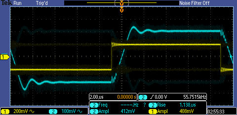
| We can see that
with a pulse wave input of .4V in yellow, the output on channel 2 has 1.138
micro-seconds for a measured rise time. This shows us that the change in
voltage per unit time is limited by the slew rate of the Opamp. The
datasheet states that the Slew Rate for the Opamp is .4V per
micro-second which coincides with our measuerd results. |
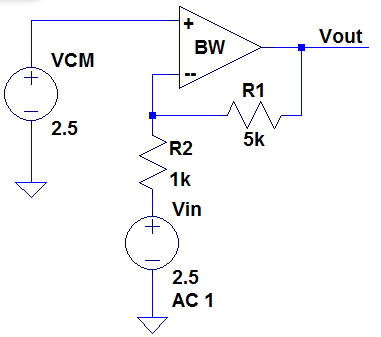
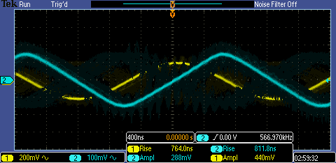
| We
can see that
with a sine wave input in yellow, the output on channel 2 has 812
nano-seconds for a measured rise time, and an amplitude of 288mV.
The saw wave output shows us that the change in
voltage per unit time is limited by the slew rate of the Opamp, and the
slew rate can be calculated as the AMPLITUDE/(RISE TIME). The
calculation for our measured results is 288mV/8212ns =
.354V/microsecond which is close the slew rate of .4V/microsecond given
by the datasheet. |
Return to EE420 labs